The article version of this write-up can be seen here!
Introduction
This is a documentation and a technical write-up for the SQL and tableau dashboard project for a real online marketplace. The dashboard created would be meant for the company’s use and tells them about the general health and potential problems that are meant to be noticed from the visualizations.
The goal of this project is to execute a dashboarding plan by creating a database pipeline with SQL and python that feeds the data that will be streamed through tableau. There are a couple of adjustments for the pipeline that were made, mainly because we are not working with an actual cloud database, instead we are working with our local storage and try our best to simulate the process.
Dataset
The dataset is taken from kaggle. It is a public dataset shared by a Brazillian E-commerce marketplace called Olist. Sellers provide their products through this marketplace, and customer can browse through various products and purchase them, then the products are sent through Olist as well to its customers. This dataset includes informations of orders from 2016 to 2018, products information, deliveries information, and product reviews. The company included the dataset structure Figure 1 along with the dataset. Out of the 8 tables included, we will only be using 7 of them. The exluded table is the olist_sellers_dataset since we are only examining the customers and deliveries in this project.
Dataset schema
Figure 1: Dataset schema
Here are some quick counts from the dataset.
Table 1: A quick glimpse into the data for reference
con.sql(f'''SELECT COUNT(*) AS total_entries, COUNT(DISTINCT order_id) AS unique_orders, COUNT(DISTINCT product_id) AS unique_products_sold, COUNT(DISTINCT seller_id) AS unique_sellers, (SELECT COUNT(DISTINCT customer_unique_id) FROM stg_customers) AS unique_customersFROM stg_order_items''')
Olist also included some notes about their datasets. They mentioned that:
An order might have multiple items
Each item might be fulfilled by a distinct seller
All text identifying stores and partners where replaced by the names of Game of Thrones great houses.
Only the first two are relevant for our purposes here, it basically says that An order entry, could contain multiple products from different sellers. This is fine and pretty expected, however we found out that there are consequences of these quirks that manifested in order reviews and in some way, order deliveries.
Order Reviews (Multiple reviews per order)
In olist_order_reviews_dataset, the reviews are tied only to order_id. This means that if an order contains multiple distinct products, we cannot establish which review belongs to which product.
Table 2: Category count for each order
con.sql(f'''WITH multiple_reviews AS ( SELECT order_id, COUNT(DISTINCT review_id) AS ref_count, ARRAY_AGG(review_score) AS scores FROM stg_order_reviews GROUP BY order_id HAVING ref_count > 1)SELECT a.*, multiple_reviews.scoresFROM ( SELECT multiple_reviews.order_id, COUNT(DISTINCT category_name) AS category_count, ARRAY_AGG(DISTINCT category_name) AS categories FROM multiple_reviews LEFT JOIN stg_order_items AS order_items ON multiple_reviews.order_id = order_items.order_id LEFT JOIN stg_products AS products ON order_items.product_id = products.product_id AND order_items.product_id IS NOT NULL WHERE order_items.product_id IS NOT NULL GROUP BY multiple_reviews.order_id HAVING category_count > 1) AS aLEFT JOIN multiple_reviews ON a.order_id = multiple_reviews.order_id''')
This is problematic because it masks which products are badly reviewed. So, we can’t really see which categories of product that are prone to bad reviews. To see how bad the damage is, let us see how polarizing the reviews betweeen the products are.
Table 3: Review score range within orders
con.sql(f'''WITH multiple_reviews AS (SELECT order_id, COUNT(DISTINCT review_id) AS ref_count, MIN(review_score) AS min, MAX(review_score) AS max, MEAN(review_score) AS mean,MAX(review_score) - MIN(review_score) AS rangeFROM stg_order_reviewsGROUP BY order_idHAVING ref_count > 1 )SELECT range, COUNT(DISTINCT order_id) AS order_countFROM multiple_reviewsGROUP BY range''')
There are 547 orders (around 0.5% of order, order count from Table 1) masked with multiple reviews and 2365 non-unique categories across all orders (2.4% of order-category rows). The numbers are small, but we would rather not rely on an arbitrary solution for these data and later decided to drop a dashboard page for categories and merge it with overview.
Table 4: Order-category level counts
con.sql(f'''SELECT COUNT(*) AS orders_category_count, SUM(is_single_category) AS single_category_count, orders_category_count - single_category_count AS multiple_category_count, ROUND((orders_category_count - single_category_count) / orders_category_count, 3) AS multiple_category_proportionFROM categories_deliveries''')
Payment vs items (Difference caused by installments)
We discovered that there are discrepancies between the payment_value from olist_order_payments_dataset and (price + freight_value) from olist_order_items_dataset. We suspect that it is caused by credit card interest and through checking the difference, we suspect that it is. Hence, we will be using values from (price + freight_value) since it fits our dashboard purposes.
Table 5: Payment total discrepancies grouped on installments
con.sql(f'''WITH payment_table AS ( SELECT order_id, ROUND(SUM(payment_value), 2)::DECIMAL(10,2) AS payment_total, MAX(payment_installments) AS payment_installments FROM stg_order_payments GROUP BY order_id)SELECT ROUND(MEDIAN(payment_table.payment_total/overview_agg.payment_total), 2)::DECIMAL(10,2) AS error_ratio_median, payment_installments, COUNT(*) AS countFROM ( SELECT order_id, SUM(price+freight_value) AS payment_total FROM overview GROUP BY order_id ) AS overview_aggLEFT JOIN payment_table ON overview_agg.order_id = payment_table.order_idWHERE overview_agg.payment_total != payment_table.payment_total AND ABS(overview_agg.payment_total - payment_table.payment_total) > 0.02GROUP BY payment_installmentsORDER BY payment_installments ''')
One interesting finding is that the same multiple product, are charged separately for its freight_value. This is very different from what we have in Indonesia and we thought that it is a very interesting finding. We see from Table 6 that there are two of the same products in this one order, and Table 7 shows that both price and freight_value sums into the total payment.
Table 6: : A specific order that have multiple of the same product
We discovered while making query for a customer retention dashboard (which we will not be making) that there are very few repeat orders within this two years interval as seen from Table 8.
Table 8: How many times customers ordered.
con.sql(f'''SELECT customers.customer_unique_id, COUNT(DISTINCT orders.customer_id) AS order_countFROM stg_customers AS customersRIGHT JOIN stg_orders AS orders ON customers.customer_id = orders.customer_idGROUP BY customer_unique_idHAVING order_count > 1ORDER BY order_count DESC''')
From around 96000 unique customers, only around 3000 customers have repeat orders. This is very small and potentially discards our customer retention dashboard plan.
Table 9: Gap between order and its next orders for each customers.
con.sql(f'''WITH multiple_orders_count AS ( SELECT customers.customer_unique_id, COUNT(DISTINCT orders.customer_id) AS order_count FROM stg_customers AS customers RIGHT JOIN stg_orders AS orders ON customers.customer_id = orders.customer_id GROUP BY customer_unique_id HAVING order_count > 1),next_order_table AS ( SELECT customers.customer_unique_id, customers.customer_id, LEAD(order_purchase::date, 1) OVER (PARTITION BY customers.customer_unique_id ORDER BY order_purchase) - order_purchase::date AS next_order_days FROM multiple_orders_count INNER JOIN stg_customers AS customers ON multiple_orders_count.customer_unique_id = customers.customer_unique_id LEFT JOIN stg_orders AS orders ON customers.customer_id = orders.customer_id QUALIFY next_order_days IS NOT NULL)SELECT customer_unique_id, MEAN(next_order_days) AS mean_next_order, MEDIAN(next_order_days) AS median_next_order, MIN(next_order_days) AS min_next_order, MAX(next_order_days) AS max_next_order, COUNT(*) AS order_count_after_firstFROM next_order_tableGROUP BY customer_unique_idHAVING order_count_after_first > 1''')
Upon further digging, we only found 252 customers out of the ~3000 customers have more than 2 orders. At this point, we decided to discard the idea of customer retention dashboard due to the small number of repeat orders. A full walkthrough of this can be seen in here.
Order status not being updated for a while.
The last of our findings is that we found orders that are not updated for a while. We do not know whether this status is true (which means some orders are stuck for hundreds of days) or false (which means some bug or systemic error). But, we cannot do anything about this, so we will leave it be and note its existence.
Table 10: Earliest and latest orders by status
con.sql(f'''SELECT order_status, MIN(order_date) AS earliest_order_date, MAX(order_date) AS latest_order_dateFROM overviewGROUP BY order_status''')
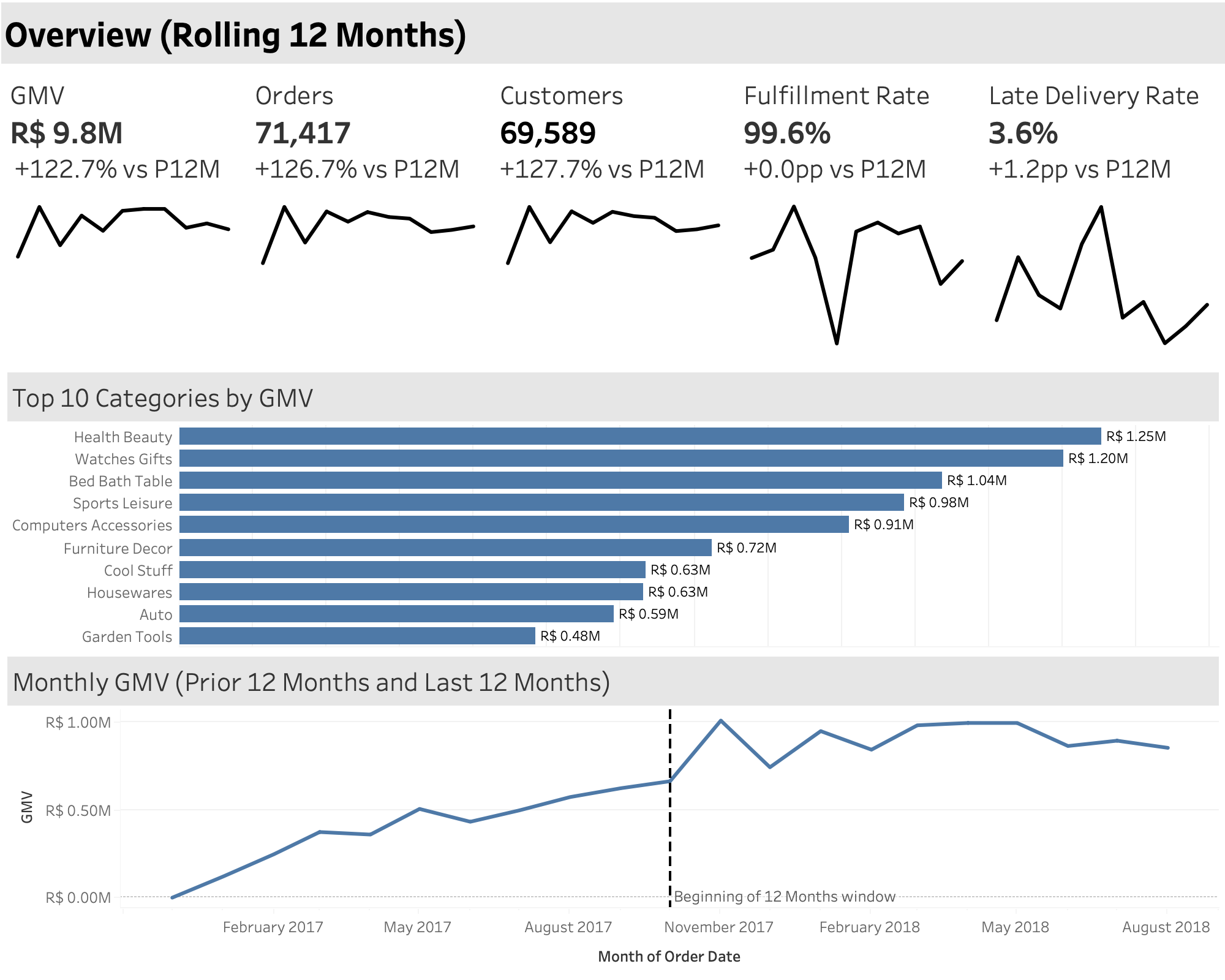
With our finddings in mind, we decided to make two dashboard pages. The first page is the overview page. It tells the viewer about the company’s health. We included metrics that indicate customers interest (Gross Merchandise Value (GMV), Total unique customers, Total unique orders, and Fulfillment rate), and logistics side performance (Late deliery rate) in a rolling 12 months window along with its sparklines in order to quickly spot trends. Then, top 10 performing categories by GMV and a lineplot of the GMV for the last 24 months are displayed to give a bit more insight.
Do note that
GMV is calculated by summing price of purchased products.
Fulfillment rate is calculated by counting how many orders are delivered over how many orders are placed and it is attributed to when the orders are placed.
Late delivery rate are orders that are late (exceed estimated delivery date given) over delivered orders.
Normally, another page dedicated to performance by categories would be created. However, due to the quirks mentioned, a focused page on categories would provide misleading informations.
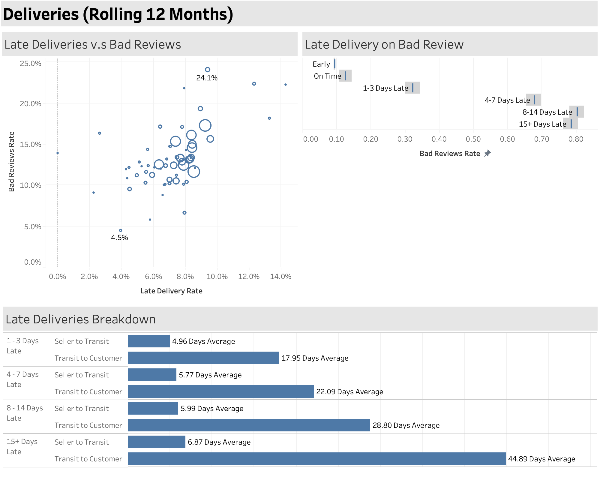
The second page wouldbe the deliveries page where we addressed the relationship between deliveries and reviews. Late deliveries are often a problem in logistics, so it would make sense to see how it would affect the marketplace business. We added a scatter plot for late deliveries against bad reviews (<= 2 star reviews), then we classify late deliveries based on how long and estimate its confidence interval against bad reviews. Finally, we added a breakdown for delivery process grouped by late deliveries classses. This would tell us, which part of the deliveries are problematic.
Pipeline
We did not do this project with cloud databases. So, we replaced it with DuckDB and local database. We attempted to replicate the process as if we were using cloud database. However, we have a limited experience on working with them so do excuse the attempt.
We had two years worth of data, so there are not a lot of them. Meaning we can have a lot more leeway in the pipeline. Specifically, we decided to make the continuous query (monthly update) to be the initial query where we reselect the entire rows. DuckDB is a column oriented database, so this decision is trivial especially when there is no partition design in our database. The pipeline is clearly visualized in Figure 2.
flowchart TB
    subgraph DuckDB
        direction TB
        Datasets --> Staging
        Staging --> Marts
        Marts --> Checks
    end
    subgraph Exports
        direction LR
        subgraph Title [ ]
            direction LR
            overview.csv
            categories_deliveries.csv
        end
        delay_ci.csv
    end

Checks --> Exports
Checks -- "Python" --> delay_ci.csv
Exports --> Tableau

style DuckDB fill:none,stroke:#333,stroke-width:2px
style Exports fill:none,stroke:#333,stroke-width:2px
style Title fill:none,stroke:#333,stroke-width:0px
Figure 2: Data pipeline from database to tableau
A walkthrough on this pipeline can be found in here. A brief explanation on the pipeline is as follows:
Staging, where we select and clean relevant columns from each tables. We also rename some columns and we decided to do join on category name translation in this stage.
Marts, where we apply business logic and output a table ready to be ingested by Tableau. Normally, there is an intermediate step before this, but we had very few marts and decided to skip that step entirely.
Checks, are list of queries that checks and make sure that the data in marts are correct and inline with its purposes. Here are the list of checks that we did.
con.sql(f''' WITH grain_overview AS ( SELECT order_id, product_id FROM overview GROUP BY order_id, product_id HAVING COUNT(*) > 1 ), grain_categories AS ( SELECT order_id, category_name FROM categories_deliveries GROUP BY order_id, category_name HAVING COUNT(*) > 1 ), missing_orders AS ( SELECT order_id FROM stg_orders WHERE order_id IN (SELECT order_id FROM stg_order_items) AND order_id NOT IN (SELECT order_id FROM overview) ), revenue_count_overview AS ( SELECT COALESCE(SUM(price + freight_value) = (SELECT SUM(price + freight_value) FROM stg_order_items), FALSE) AND COALESCE(SUM(item_count) = (SELECT COUNT(*) FROM stg_order_items), FALSE) AS pass_check FROM overview ), revenue_count_categories AS ( SELECT COALESCE(SUM(price + freight_value) = (SELECT SUM(price + freight_value) FROM stg_order_items), FALSE) AND COALESCE(SUM(item_count) = (SELECT COUNT(*) FROM stg_order_items), FALSE) AS pass_check FROM categories_deliveries ), deliveries_statistics AS ( SELECT order_id FROM categories_deliveries GROUP BY order_id HAVING COUNT(DISTINCT review_score) > 1 OR COUNT(DISTINCT delay_days) > 1 OR COUNT(DISTINCT order_status) > 1 OR COUNT(DISTINCT is_single_category) > 1 ) SELECT 'grain_overview' AS check_name, COUNT(order_id) = 0 AS pass_check FROM grain_overview UNION ALL SELECT 'grain_categories' AS check_name, COUNT(order_id) = 0 AS pass_check FROM grain_categories UNION ALL SELECT 'unexplained_missing_orders' AS check_name, COUNT(*) = 0 AS pass_check FROM missing_orders UNION ALL SELECT 'revenue_count_overview' AS check_name, pass_check FROM revenue_count_overview UNION ALL SELECT 'revenue_count_categories' AS check_name, pass_check FROM revenue_count_categories UNION ALL SELECT 'deliveries_statistics_check' AS check_name, COUNT(*) = 0 AS pass_check FROM deliveries_statistics ''')
Recall that we have problem regarding multiple reviews within the same order. We decided to take the earliest review. This decision is arbitrary but we have no justification to do otherwise.
Exports, normally this is unnecessary, but since we are using local database, we had to export the results so Tableau can ingest.
We executed all these steps using a shell script that exits if there are errors (which Exports should throw if there are any) in any part of the pipeline. Do check the shell script in the project repository
In addition to using the marts in Tableau, we also did a proportion z-test for one component of the dashboard using the exported marts.
Result and Insights
Overview Page
Olist overview dashboard — click to explore the interactive version on Tableau Public
From this snapshot, we can see that GMV, Customers, and Orders are plateauing despite the massive increase compared to the prior 12 months. Prompting to ask a question regarding the reason why the growth on number of orders fell. Perhaps it signifies an end to a certain stage in the business or the market being saturated. Then, another metric to pay attention to is the late delivery rate. 3.6% for the last 12 months is not bad, but upon further inspection, there is a spike in March 2018 that reached 19% late delivery rate. It should be investigated why this happens and what are the effects on the marketplace which would lead to the deliveries page.
Additional graphs below gives us what categories contributes the most to our GMV and a broader overview on GMV for the last 24 months.
Deliveries Page
Olist deliveries dashboard — click to explore the interactive version on Tableau Public
Here, the scatter plot shows some correlation between late deliveries and bad reviews. Then, we quantify this correlation with the confidence intervals for every delivery time against bad reviews rate. We can see that later deliveris is associated with more bad reviews, but after 8-14 days late, the increase in bad reviews are relatively small compared to jump from other intervals. While it is just an association from this visualizations, it still warrants further investigation as the possibility of bad reviews caused by late deliveries hurts the sellers.
Finally, we want to see what happened during deliveries, and the bottom chart shows what happened. Sellers seems to deliver their products around 4-6 days, while the logistics takes much longer to deliver to the customers. It also increases as the delivery time increases. A further investigation on to the logistics must be done at this point.
Project Recommendations
To reiterate, the insights that we get from these dashboards is that,
Market growth is plateauing
Late deliveries are associated to bad reviews, the later, the higher the rate of bad reviews. Increases significantly up until 8-14 days late where the increase is relatively small.
Late deliveries mainly takes a lot of time during logistics to customer phase.
Therefore, we would recommend from these dashboards to do reasearch on the reason why growth is plateauing. Also, investigate the problem within the logistics in order to reduce bad reviews that are placed on the sellers. We should investigate how bad reviews affect products as well because it might deter away sellers from the marketplace.
The article version of this write-up can be seen here!