── Conflicts ────────────────────────────────────────── tidyverse_conflicts() ──
✖ dplyr::filter()       masks stats::filter()
✖ purrr::flatten()      masks jsonlite::flatten()
✖ lubridate::interval() masks tsibble::interval()
✖ dplyr::lag()          masks stats::lag()
ℹ Use the conflicted package (<http://conflicted.r-lib.org/>) to force all conflicts to become errors
library(ggplot2)library(rvest)
Attaching package: 'rvest'

The following object is masked from 'package:readr':

    guess_encoding
library(imputeTS)library(scales)
Attaching package: 'scales'

The following object is masked from 'package:purrr':

    discard

The following object is masked from 'package:readr':

    col_factor
The API call only returns data from 2024, so downloading the excel file from the website is recommended. The dataset is taken from https://satudata.jakarta.go.id/open-data/detail?kategori=dataset&page_url=jumlah-penumpang-angkutan-umum-yang-terlayani-perhari&data_no=1
during the time of analysis, the latest data is at 2026-04-30.
# API Calldf <-read_html("./data/jumlah-penumpang-angkutan-umum-yang-terlayani-per-hari-komponen-data.xls") %>%html_table()# To csvwrite.csv(df, "./data/daily_transport.csv", row.names=FALSE)# CSV if existdf <-read.csv("./data/daily_transport.csv")df %>%head(5)
  periode_data    tanggal jenis_moda jumlah_penumpang_per_hari
1       202402 2024-02-25      KAPAL                      4535
2       202402 2024-02-26      KAPAL                      1830
3       202402 2024-02-27      KAPAL                      1673
4       202402 2024-02-28      KAPAL                      1479
5       202402 2024-02-29      KAPAL                      1477
Noted that some data in jumlah_penumpang_per_hari contains , as a delimiter and messes up the integer conversion.
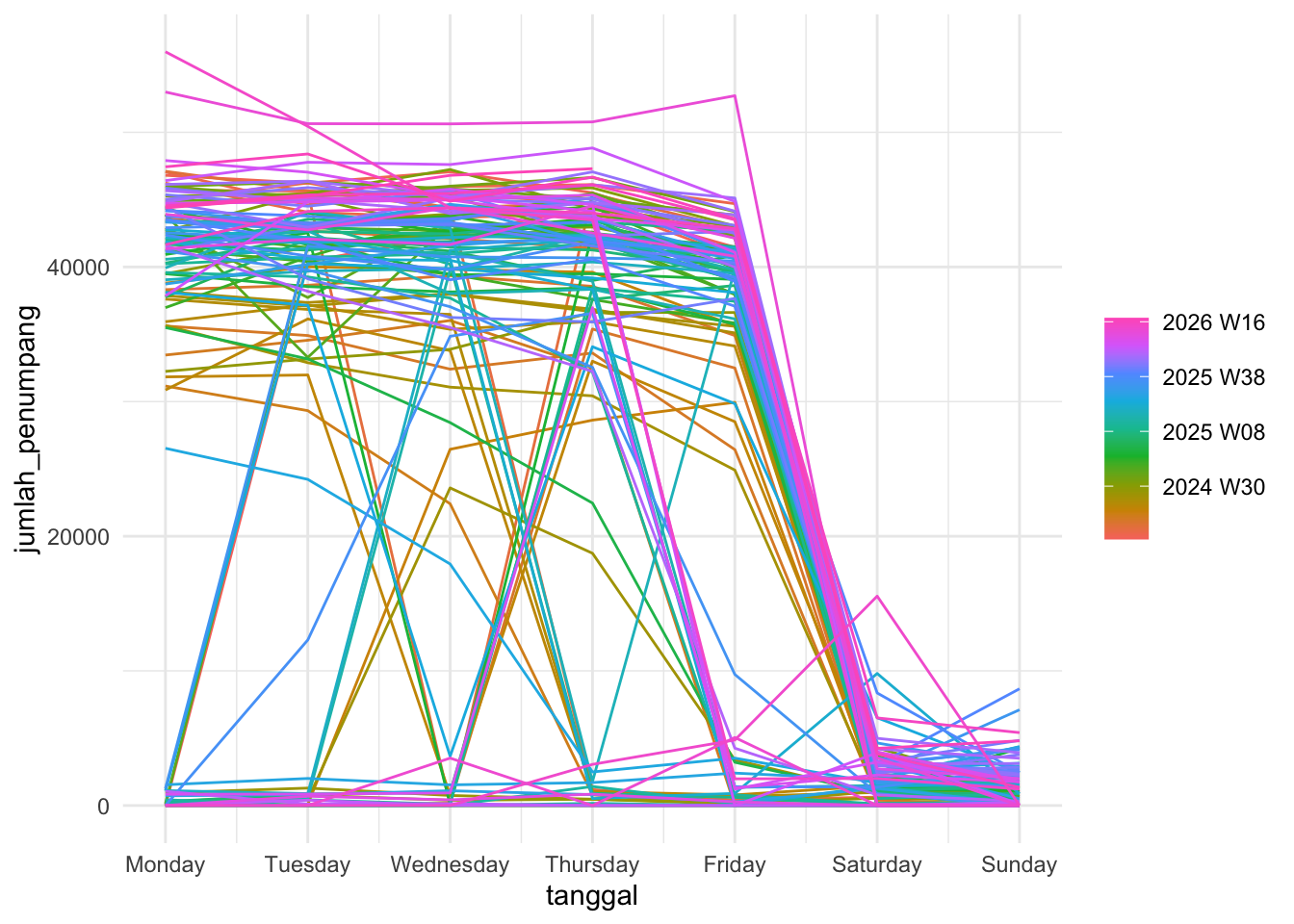
There are a lot of weeks in here so it looks really cluttered in the operational interval. But, it is clear that the value dips in Saturday and Sunday.
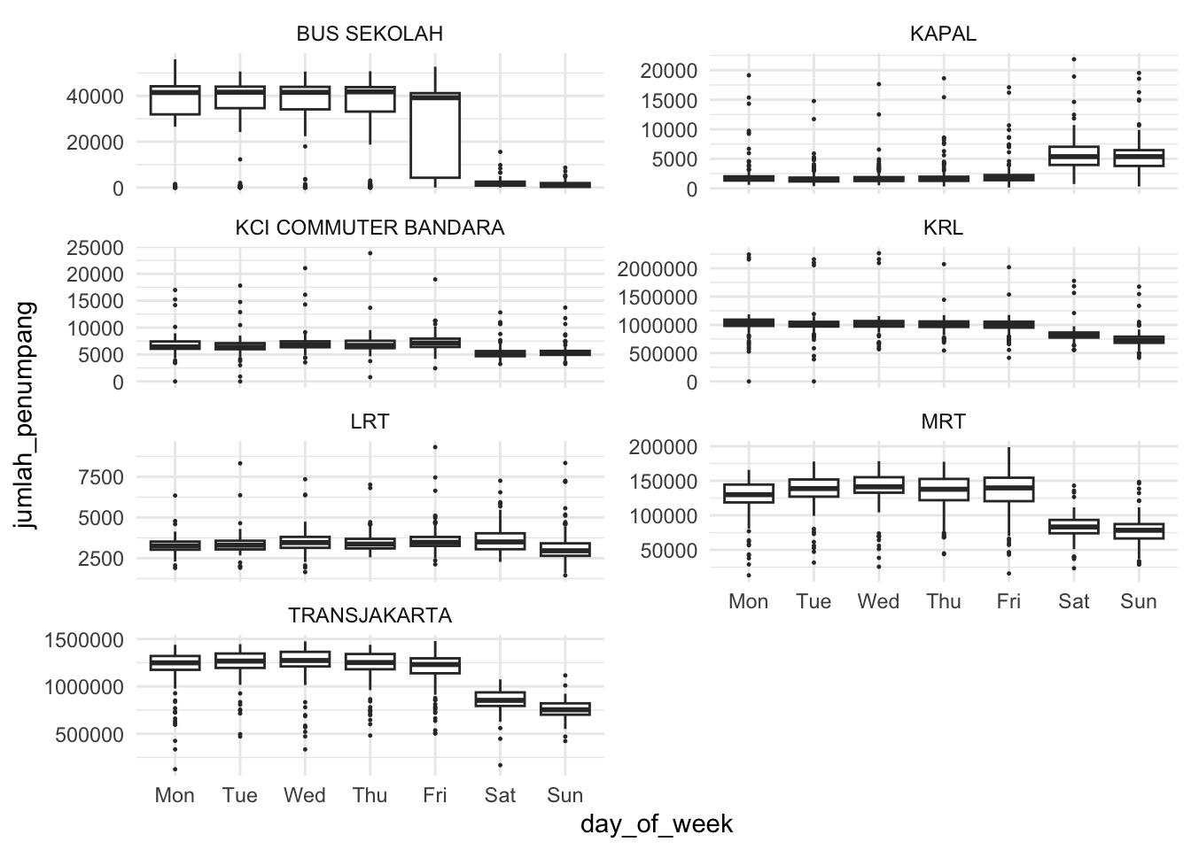
Hence, we will use a boxplot in order to smoothen things and we can see some general pattern for each transportation methods.
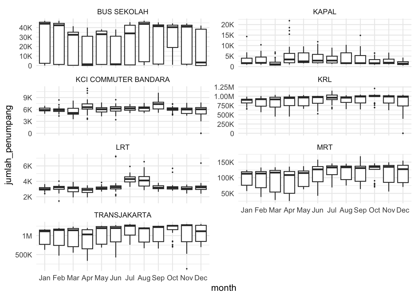
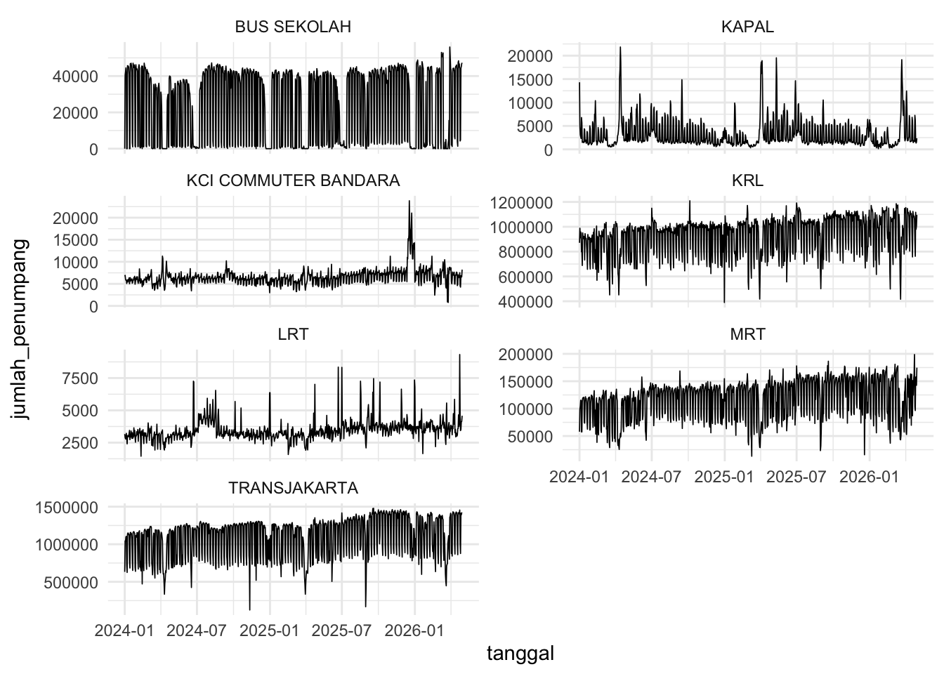
There is no pattern here, except that there are times where BUS SEKOLAH are zero’d because of school holiday. KAPAL shows a lot of outliers, presumably because of Eid. KCI COMMUTER BANDARA have a small amount of passengers and a lot of outliers so it might be hard to model. Finally, LRT as mentioned previousy, does not show weekly pattern. Hence, for modelling, we will focus on KRL, MRT, and TRANSJAKARTA.
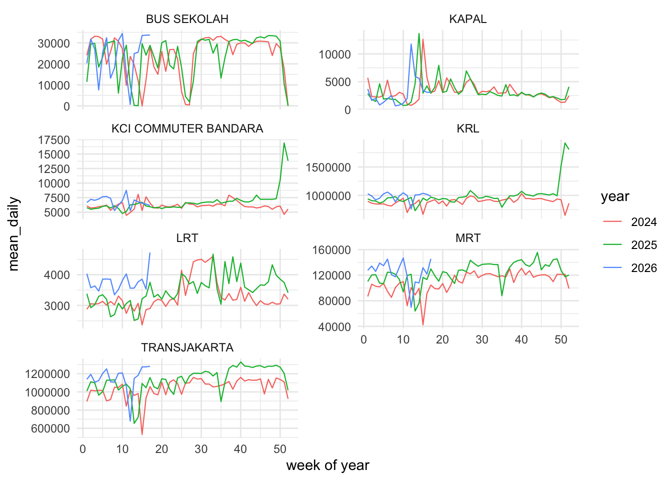
We can see that a lot of transport shows a dip during Eid while KAPAL and KCI COMMUTER BANDARA have a spike during that time, which makes sense because people tend to travel far during that time. Recall that this is transport data for Jakarta, meaning that a lot of people that stayed in Jakarta, are not actually from there.
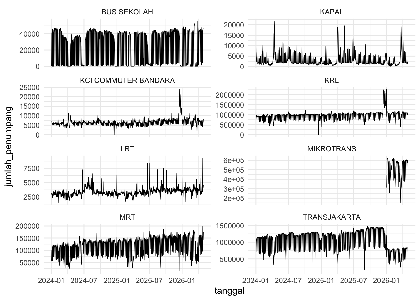
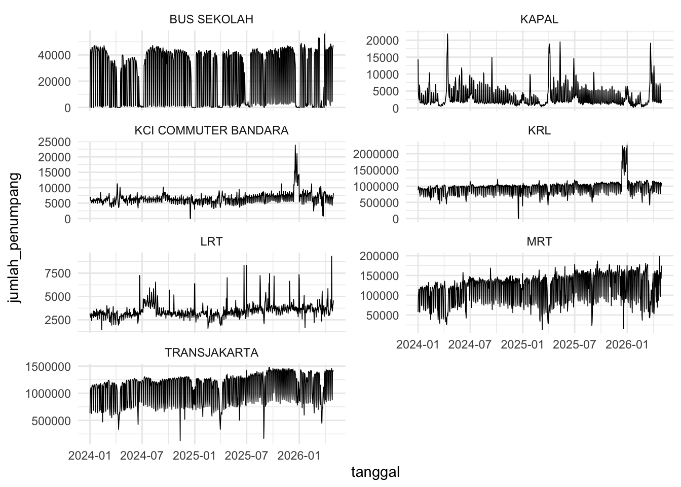
Very high spike for end of year for both KRL and KCI COMMUTER BANDARA. This does not look normal, especially since the year before that, there is a slight dip. This warrants further investigation.
Anomaly on KRL and KCI
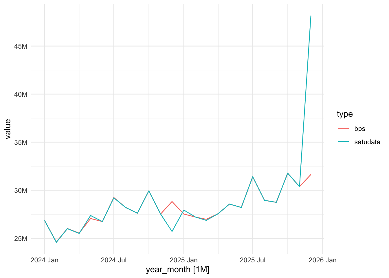
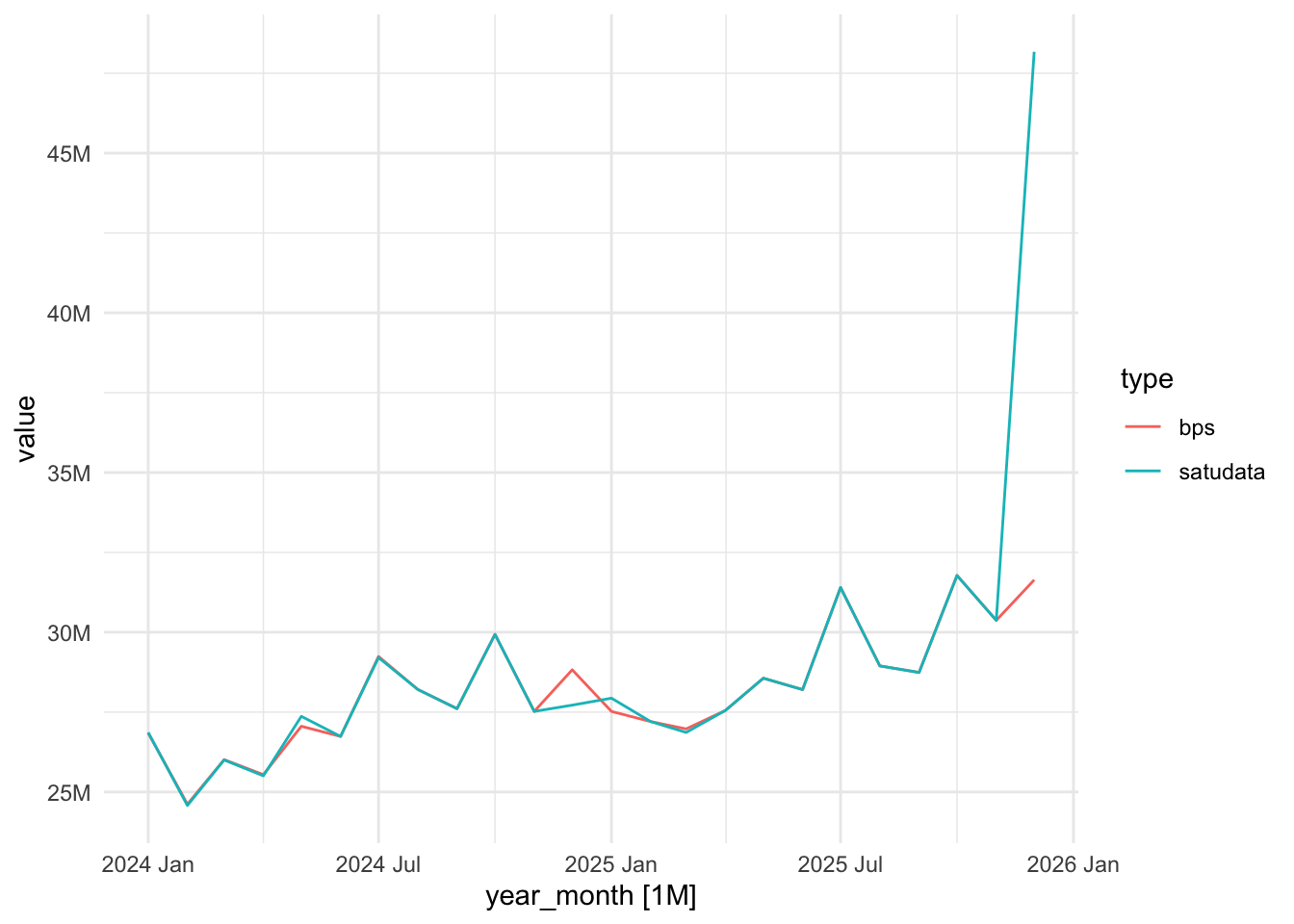
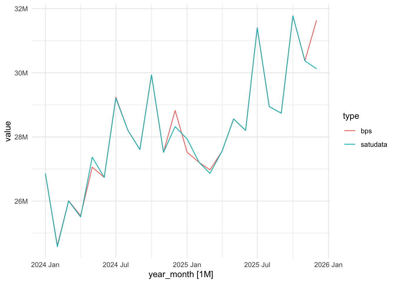
https://www.bps.go.id/id/statistics-table/2/NzIjMg==/jumlah-penumpang-kereta-api.html Total for Jabodetabek in December is actually 31640000 according to this website. So, let us check the dataset against these statements. While we are at it, we will also check for every month as well.
For December 2024 deviation, the dataset actually understates compared to BPS, which is why we have the dip earlier. Recall that when checking for 0 total passengers, KRL and KCI does have two entries that are zero in December 2024. Imputation will be done since a gap in the middle of dataset is really troublesome.
Two statements from this news 1. “18 sampai 25 Desember 2025 sebanyak 7.839.814” Passengers from 18 - 25 December 2025 totals 7839814. 2. “PT KAI Commuter Indonesia (KCI) mencatat jumlah penumpang Commuter Line atau KRL Jabodetabek mencapai 724.536 orang pada libur Natal 2025, Kamis (25/12/2025)” Total passengers in 25 December 2025 is 724536
Let us perform a time series decomposition, to see the seasonality and trend clearly for the three chosen methods of transport that we want to model. But first, let us mark Eid dates.
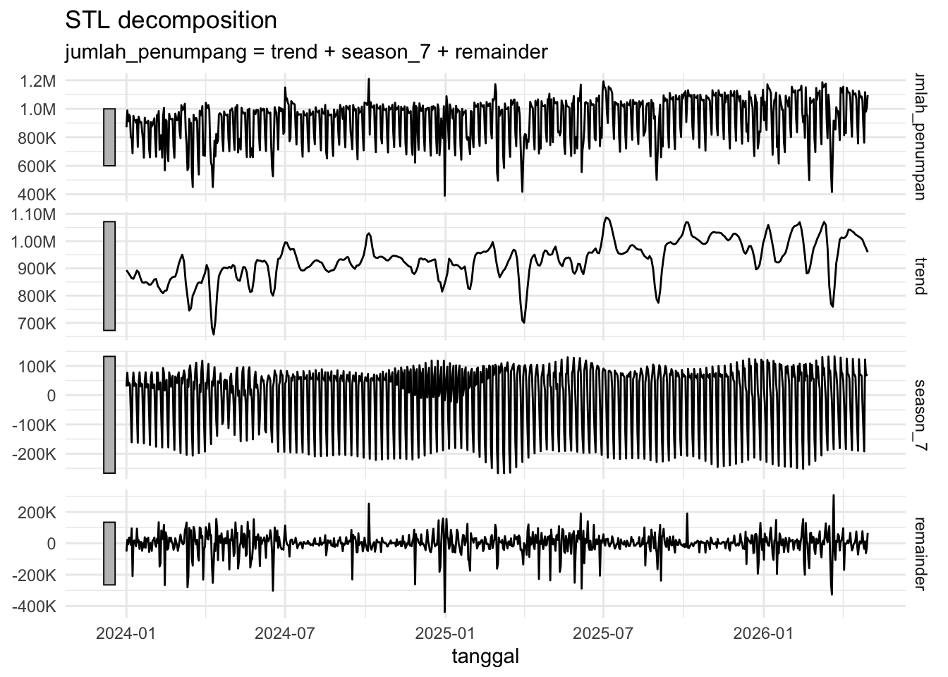
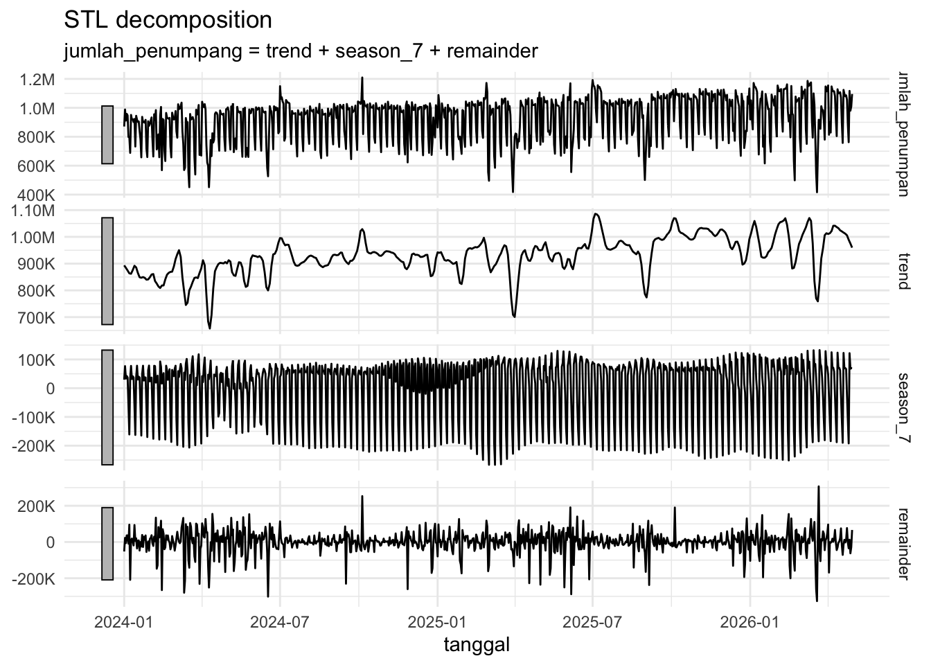
There is a very sharp dip at 2025-01. Recall that there was an imputation at 2024-12 but after checking with BPS data, it is still understated. It seems that we still need to check the numbers around that area again.
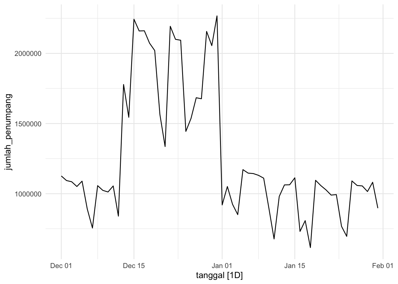
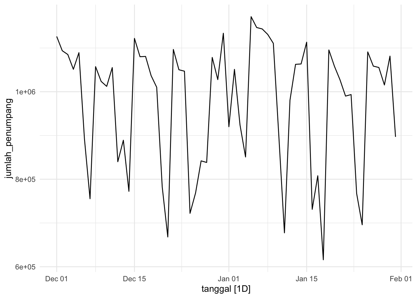
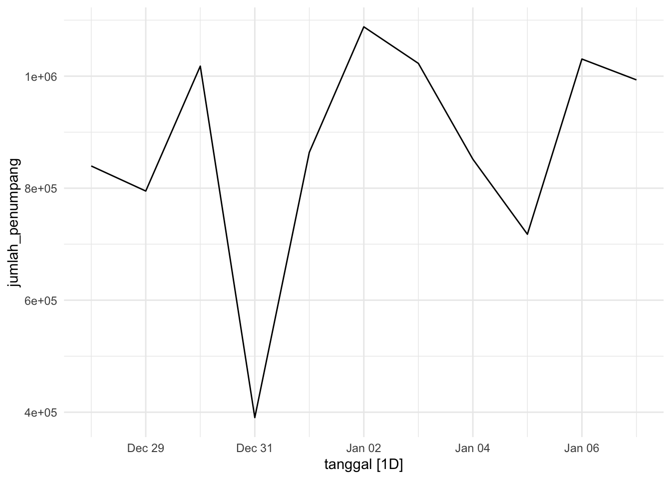
df_clean %>%filter(tanggal >="2024-12-28", tanggal <="2025-01-07", jenis_moda =="KRL") %>%select(tanggal, jumlah_penumpang) %>%autoplot(.vars=jumlah_penumpang)
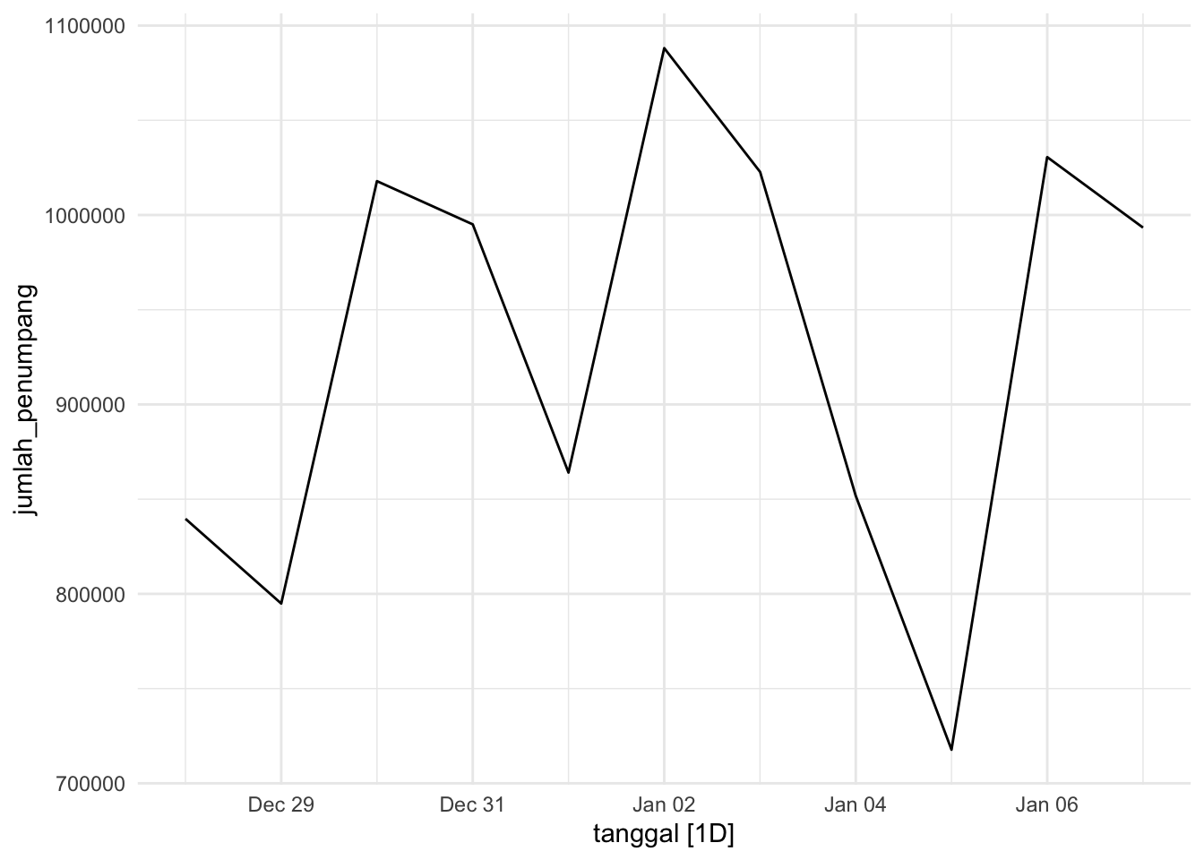
Seems like we missed an anomaly, December 31st is so low compared to the others. It doesn’t make sense, since KRL operational hours is extended during new year’s eve. Since we don’t have any validation, we will set the value to NA and impute it.
This is a one-off and honestly, it is quite difficult to handle since we cannot predict these demonstrations reliably. Hence, this interval will be left as is, and noted that it might ruin the model fitting.
We can see that the trend still captures some sharp dips that is probably attributed to Eid. This decomposition cannot adjust for that since we stated that we only have weekly seasonality.
We see that there is no structure left in the remainder, meaning we captured most if not all of the seasonality pattern.
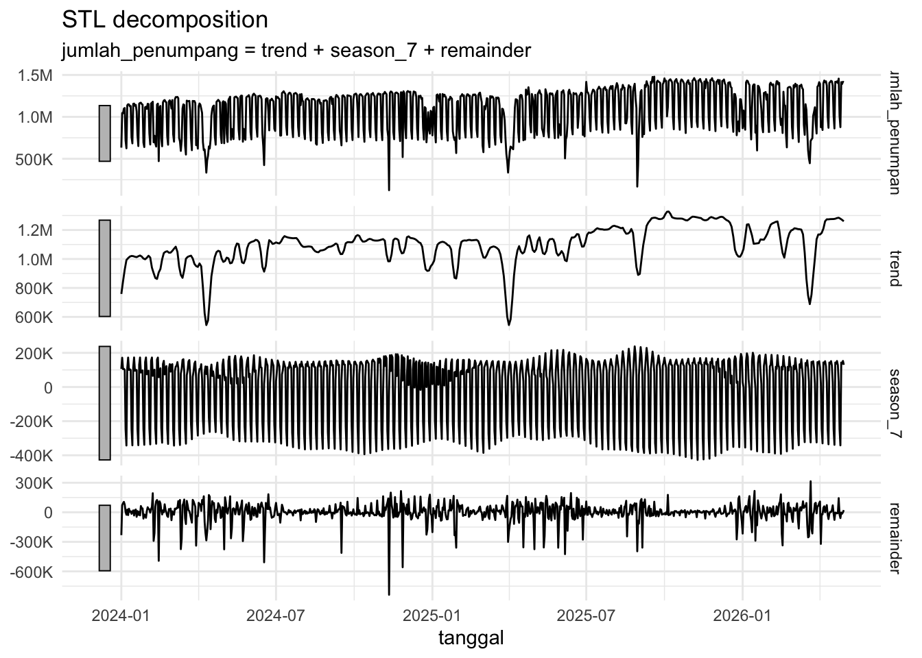
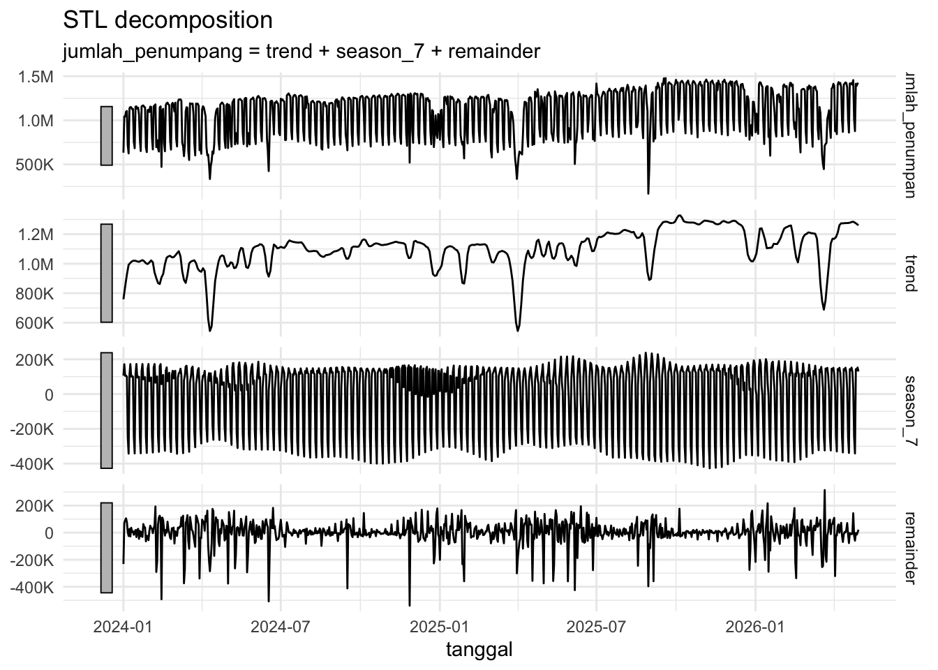
Similar to KRL, the trend absorbed some events that happened throughout the timeline. That includes Eid, and the Riot. There is a sharp dip in the end of 2024 though, so let us check if it needs to be handled.
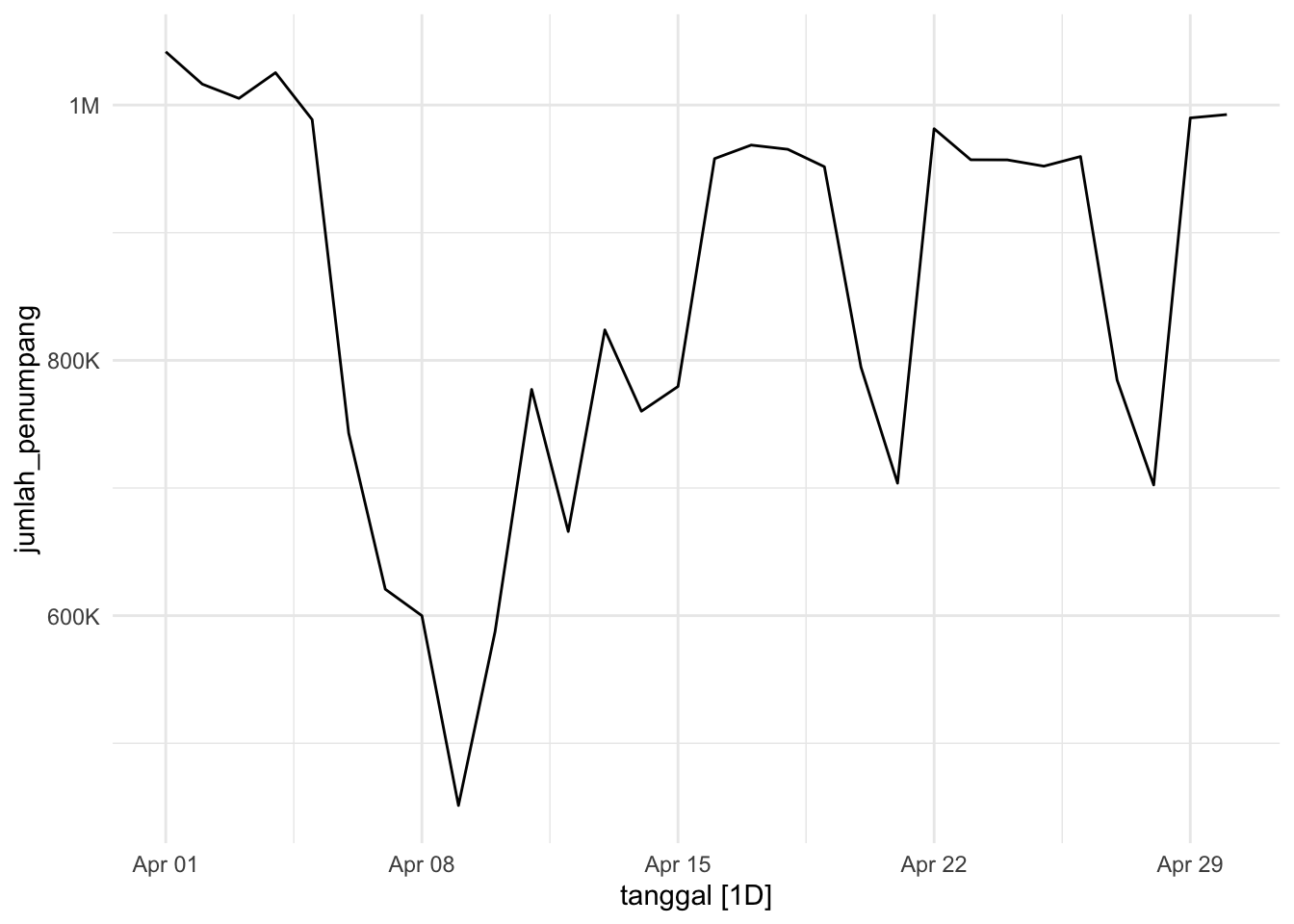
There is a sharp dip in 2024-11-11. I have no idea what could caused it, but I see that there is a route change that happens in that time.
https://www.instagram.com/p/DCG1_82y070/
But, it seems that it is way too low of a decrease for it to be caused by two route changes. Besides, it’s not like the transportation itself stopped operating, so one might think that this is some kind of system error.
Then, there is another dip in 2024-11-27, which might be caused by regional elections and TRANSJAKARTA only operates from 09:00 AM instead of 05:00 AM.
The first dip might warrant some intervention while the second dip should be left alone and noted.
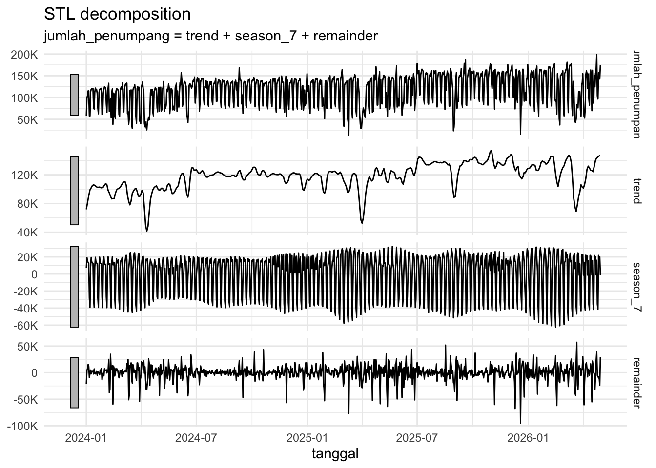
MRT looks really stable. Again, the four previously identified dips appeared. There is nothing to change or to check so we left it as is.
Final Check
There are a lot of unexpected anomalies that required imputations that refers to other dataset. Here is the list of what was imputed
jumlah_penumpang that have 0 for KRL and KCI COMMUTER BANDARA (2024-12-16, and 2024-12-17) are imputed using na_seasplit()
jumlah_penumpang at 2024-12-31 for KRL is replaced with NA and imputed using na_seasplit().
jumlah_penumpang at 2025-12-13 - 2025-12-31 is halved for KRL
jumlah_penumpang at 2024-11-11 for TRANSJAKARTA is low for unknown reason. The valued was replaced with NA. and and imputation method was implemented using na_seasplit()
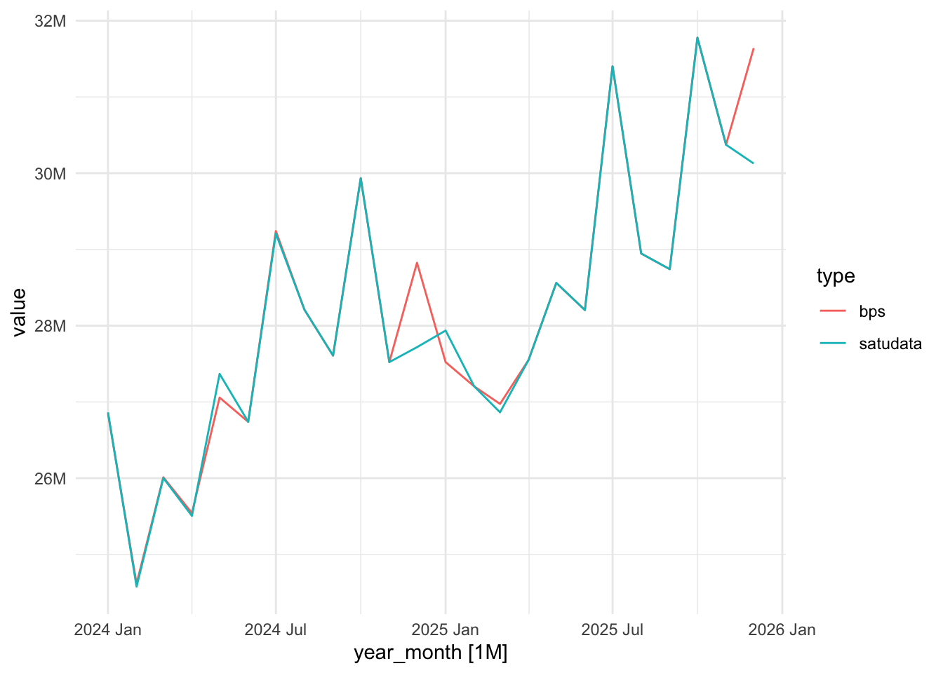
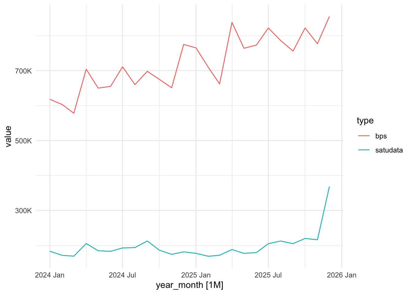
First, we want to see whether the zero values have been imputed properly for both KRL and KCI COMMUTER BANDARA. We can check the first three imputations by just comparing with the BPS data again.
Well, I suppose there is a fundamental difference between how Satudata and BPS defined it. So, we can’t really check.
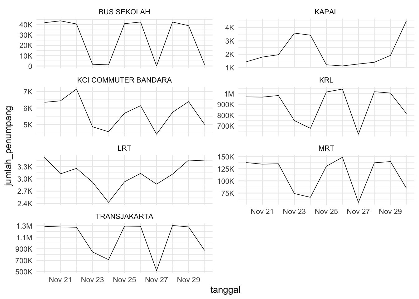
We mentioned that there is a regional election at 2024-11-27 and it does affect TRANSJAKARTA total passengers due to reduced operational hours and holiday. Does it affect other transport as well?
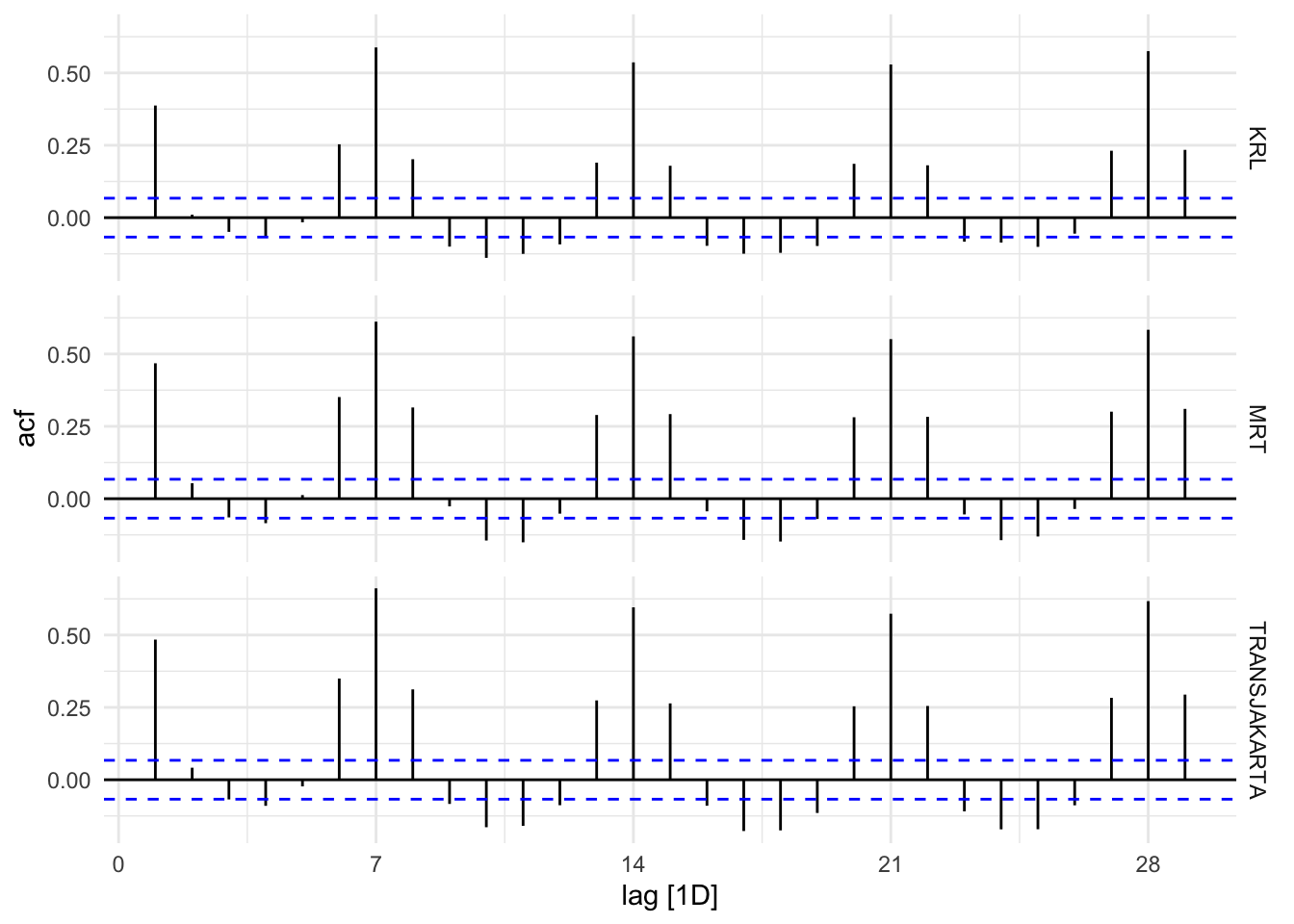
For modelling purposes, we confirmed that there is a seasonal component with 7 days period (weekly) as shown for all three jenis_moda.
Summary
We have found some interesting findings throughout the analysis. We noted some things and adjusted the data for others. Here are some findings that led the decision to adjust the data.
First, we saw that MIKROTRANS starts at the same time as when there was a chunk of data missing from TRANSJAKARTA. Hence, we decided to just merge them together.
Then, we checked for 0 values and found that BUS SEKOLAH has 81 entries that are 0 which we left as is, and both KRL and KCI COMMUTER BANDARA has 2 entries that are 0 at the same date, which we impute.
We found a sharp spike of total passengers for both KRL and KCI COMMUTER BANDARA at 13 - 31 December 2025. We validated this finding for KRL through a BPS dataset and some news articles. We decided to divide the total passengers at that time period by half since it the value looks doubled. Nothing was done for KCI COMMUTER BANDARA.
On the contrary, in 31st December of 2024, there is a sharp dip. We found no reason why this is the case, but we decided to multiply the total passengers by 2 and the result looks fine after.
There are events that happened throughout the year. Those events are considered to be a part of the model if it happens at a predictable interval, or kept as is if it is a random occurence. One event that happens every year is Eid. For that event, every transportation method except for KAPAL and KCI COMMUTER BANDARA took a dip.
Another notable event is the riot that happened from 25 August 2025 until 9 September 2025. The dip does not happened at that exact interval but somewhere within. That is caused by some stations stopped operating completely.
Lastly, there is a public holiday for a regional election in Jakarta at 2024 November 27. Every transportation method took a dip for that day.
One finding about seasonality is that almost all of the transportation method have a weekday and weekend pattern. BUS SEKOLAH stops operating at weekends, KAPAL have an increase of passengers during weekends, and the rest have a decrease of passengers during weekends except for LRT which does not seem to show any weekly seasonality.
Looking at yearly seasonality however, there are barely any visible pattern. We can only see an increase in outliers for KAPAL and KCI COMMUTER BANDARA during Eid. However, the total passengers is quite low to begin with. There are times where BUS SEKOLAH are zero’d because of school holiday. Finally, LRT as mentioned previousy, does not show weekly pattern. Hence, for modelling, we will focus on KRL, MRT, and TRANSJAKARTA.
Models
KRL
First Pass
Before we commit to cross validations, let us take a peek and maybe find out some hyperparameters if applicable.
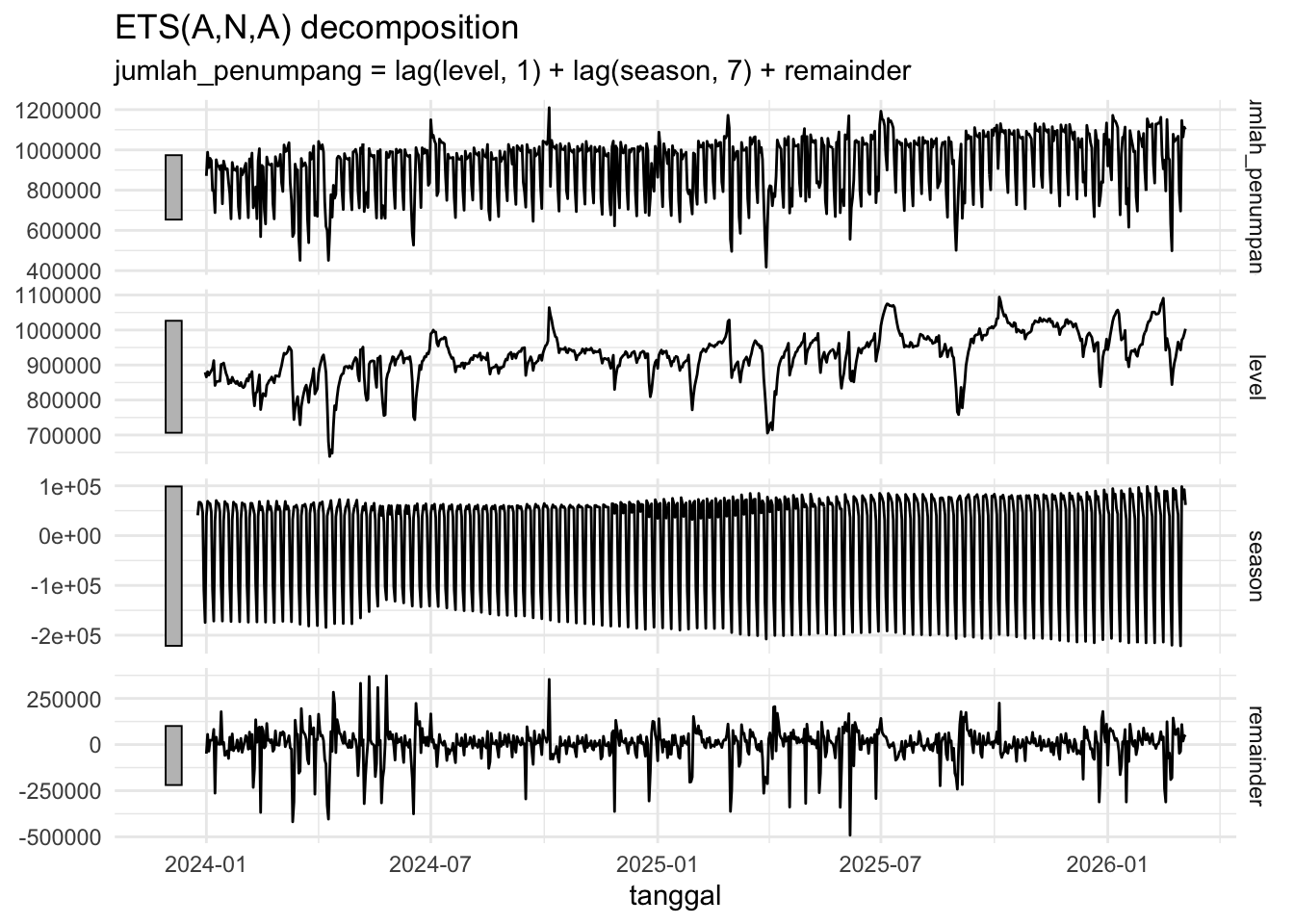
The smoothing parameters that were picked explains the decay of level and seasonality components. Alpha explains the decay of the level component, meaning the value from previous day are scaled by 0.269 and carried by the current value. Meanwhile, the gamma explains the seasonality component. The value is so small, but it explains how the value from previous season (last week) affects the current value.
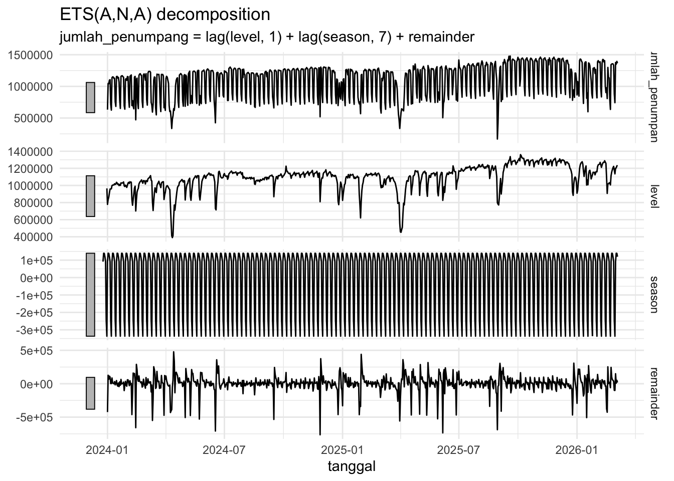
The model picks additive error, no trend, and additive seasonality. The reason additive was chosen for error and seasonality term is most likely because these two does not grow as time goes. Meaning, the fluctuations that came from the weekly seasonality does not grow bigger as time goes on, and that also applies for the error term.
The model decides an SARIMA model with parameters - Autoregressive of order 2 - Seasonal autoregressive of order 1 at lag 7 - Seasonal differencing of order 1 at lag 7 - Seasonal moving average of order 2 at lag 7
Autoregressive of order 2 suggest that the non-seasonal component of the model depends on the past two values.
The seasonal differencing of order 1 basically strips down the seasonality pattern, and the order 1 says that once the changes between the current and last season (in this case, same day of last week), the time series becomes stationary. In simpler terms, the seasonality is constant.
Seasonal autoregressive of order 1 says that the current value depends on the last season value (last week’s value), and the seasonal moving average of order 2 suggest that the current value is affected by the last two season shocks (noises).
However, it is important to note that some coefficients include 0 because of the standard error. Both the first order of the seasonal autoregressive and 2nd order of the seasonal moving average have a larger standard error than their value. Meaning, these coefficients might not be significant, but is still included because it still did improve AICc, which is the selection criterion used.
Adding a regressor term for Eid did change the model parameter slightly. Instead of seasonal autoregressive of order 1, it is now of order 2. Meaning, it argues that the model adjusted its dependence from just the last season to the last two season. However, some of these components have a large standard errors that exceeds their coefficients. In this case, - The second order of autoregressive - The seasonal autoregressive components - The seasonal moving average components
Meanwhile, is_eid component says that during eid, the passengers on average decreases by 157K with 27K standard error. So, having is_eid regressor term, weakens more components and may allow us reduce the components for a simpler model. This will be investigated further.
Compared to the previous model with 20207.37 AICc, we now have 20204.39. This is caused by the code actually used a greedy algorithm to find the best model. So, not only, it has a smaller criterion, it is also a simpler model. We will use the seasonal naive as a baseline, ETS as the next best model, and SARIMA(1,0,0)(0,1,1) as the best model and do cross validation.
Model Validation
Let us peek at how the model performs through its residuals. It is not necessary, but it is nice to see whether the model captures the structure of the data or not.
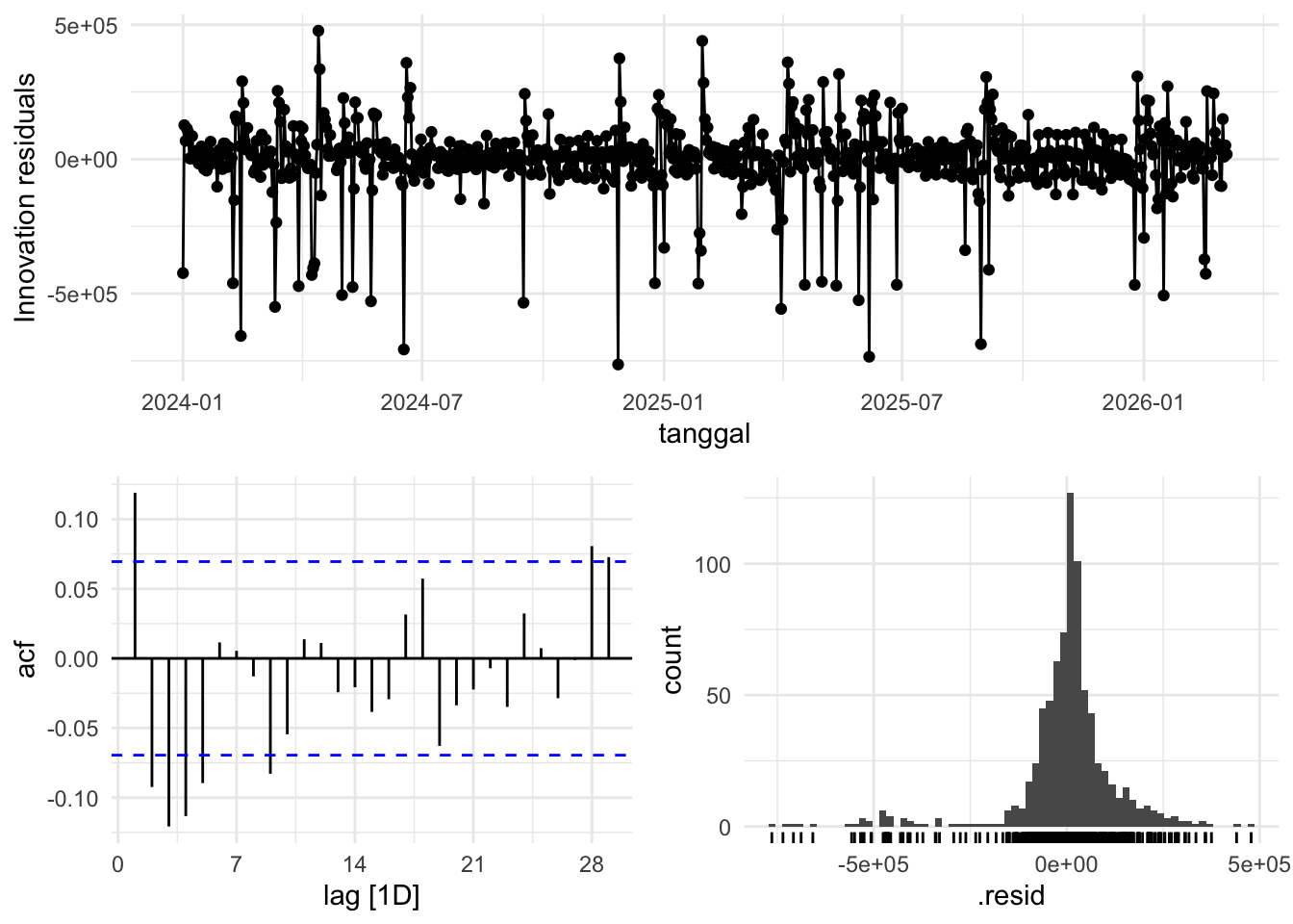
fits_krl %>%select(c(snaive)) %>%gg_tsresiduals()
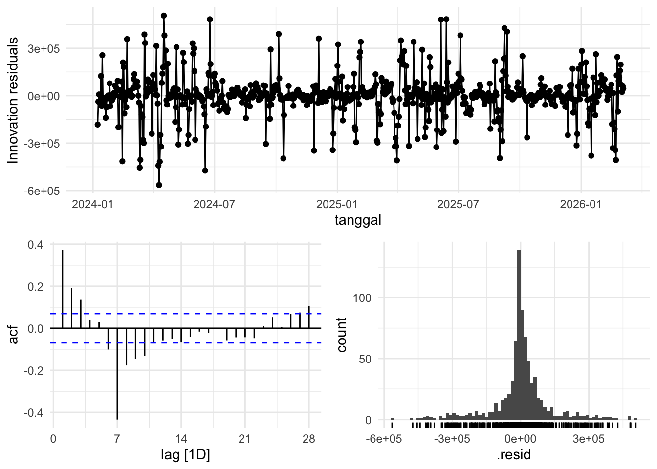
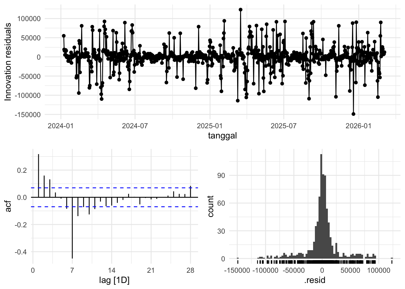
The first plot, the innovation residuals seems pretty cluttered. But, recall that we have identified events that affected the total passengers greatly. We see that early 2024, a lot of fluctuations in the residuals, which coincides with 2024 Eid timing. Then, the fluctuations starts again early 2025, and spikes after 2025-07 point, where the riot happened. Then, 2026 Eid also shows some fluctuations. It is expected that the model could not capture these events, and hence the residuals are affected during those events.
The second plot to look at is the ACF. It explains the autocorrelation for the residuals. We still have a strong autocorrelation at lag 1, which means that the residuals at current time is still correlated to the previous time. In other words, the model did not fully capture the relationship between current time and previous time (yesterday). The same can be said for lag 7, which is last week.
Also, we would like for 95% of the autocorrelation to be below the dashed blue line because that would imply that the residuals are within the 95% confidence band of white noise. In this case, we see a lot of lines crossed the blue line, and can safely conclude that the residuals are not white noise.
Finally, the residuals density plot. We can see that it is bell shaped, but it has long tails, so it doesn’t really fit the normal distribution. Let us continue with the other models briefly.
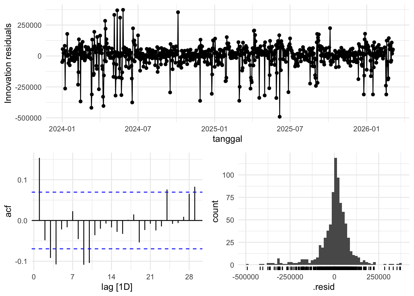
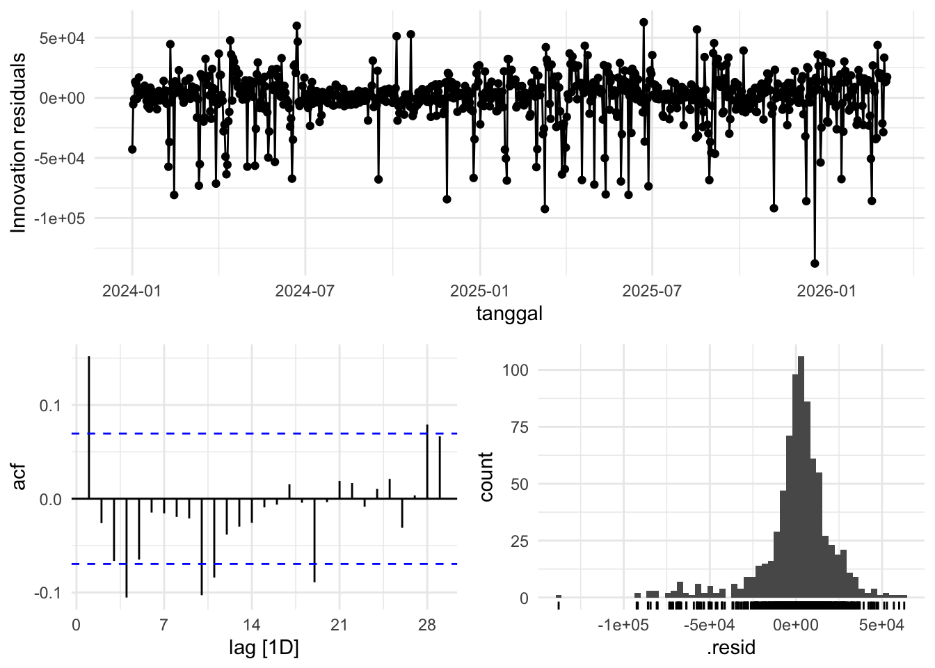
fits_krl %>%select(c(ets)) %>%gg_tsresiduals()
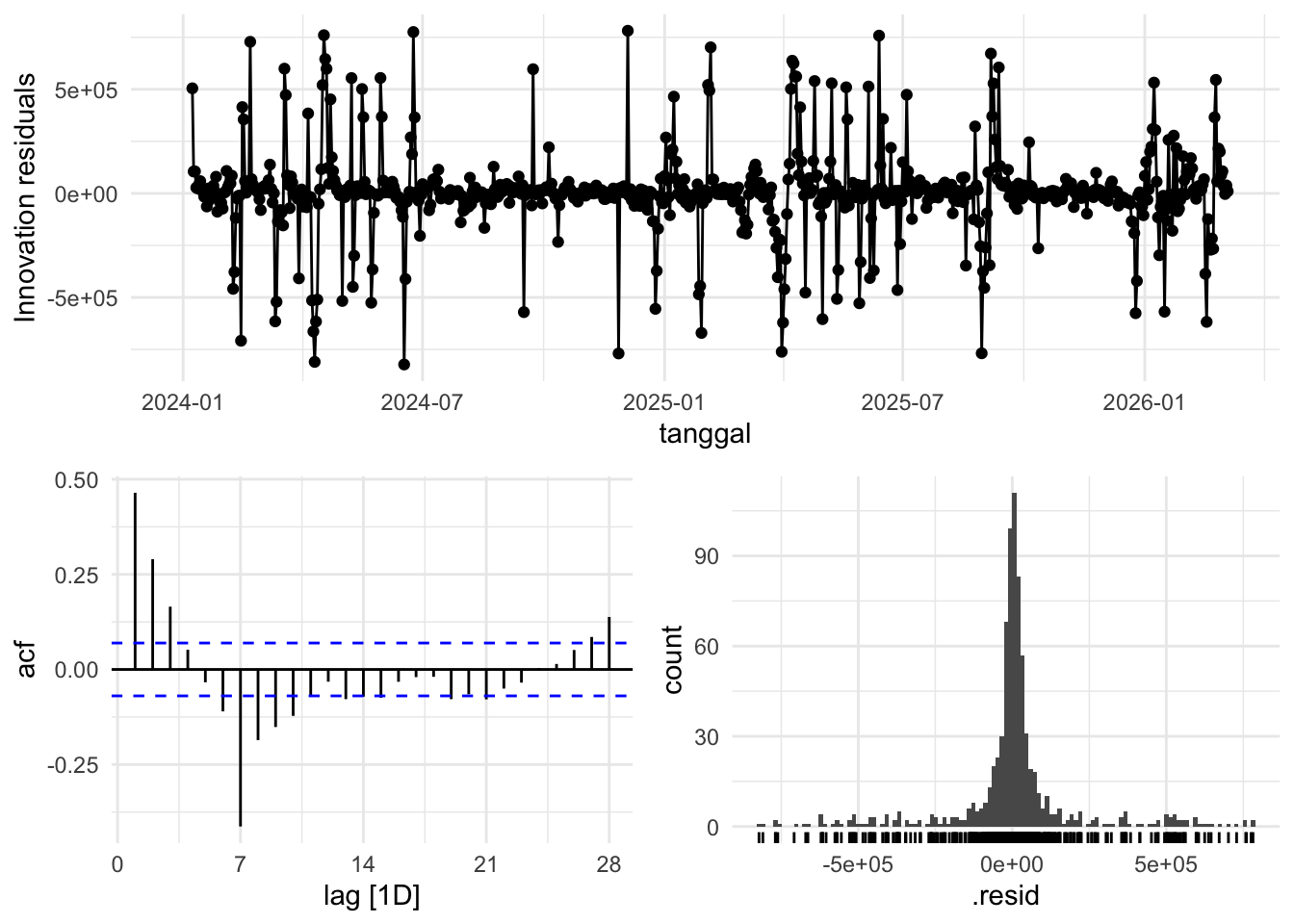
Again, fluctuations can be seen during event timings, although after 2024 events, most of the residuals went into the negative, meaning that the prediction overstates during that time. Expected since the model did not know any of these events. The ACF plot still have a strong autocorrelation for lag 1, but have no strong weekly correlation since it is captured by the seasonality component of the model. Lastly, the density plot shows that it has a long left tail, because the model overestimates during events.
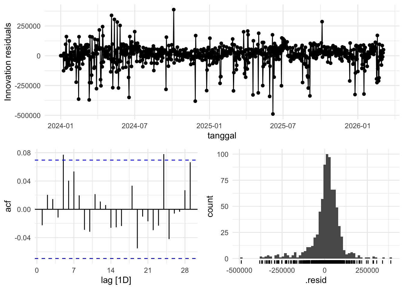
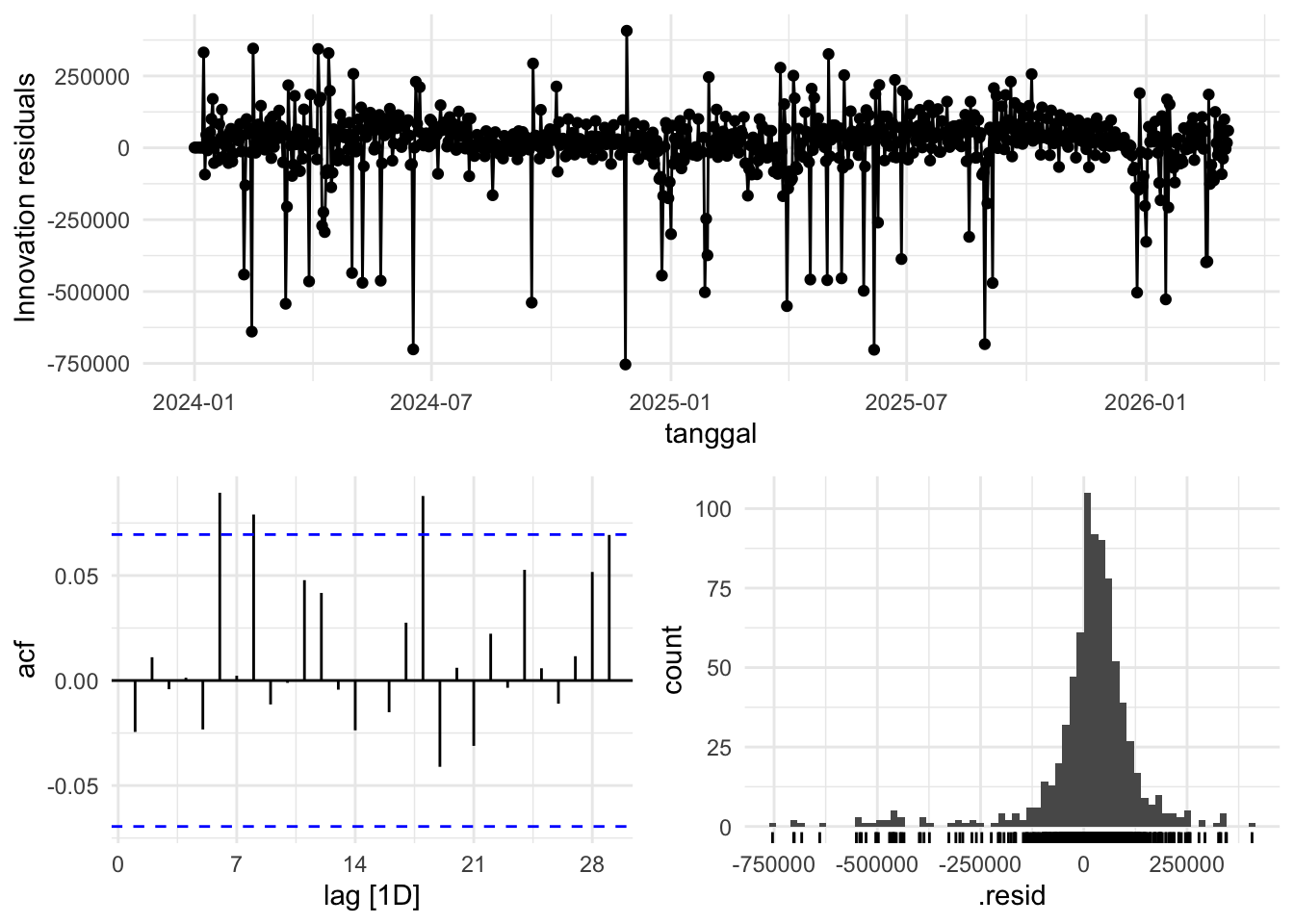
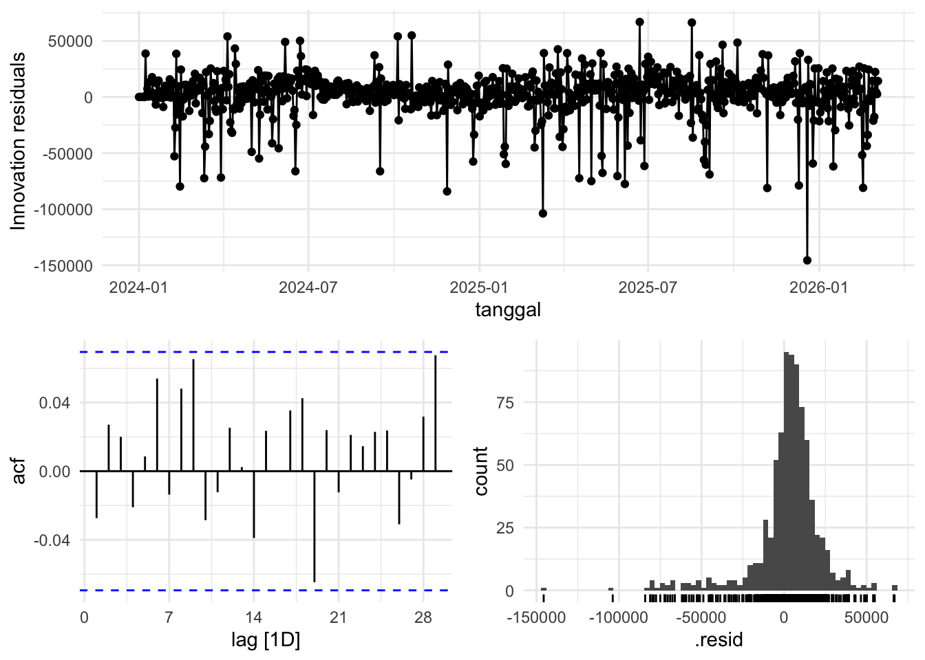
The innovation residuals looks pretty similar with ETS model despite having a regressor term for Eid. The only visible difference is that for earlier time, during 2024, this model did slightly better than ETS. The ACF plot have spikes at random lag, which we could not attribute to anything. Not to mention, there are only 2 lines out of 28 that exceeds the blue line. It is still not enough to be stated as white noise considering this plot. Next, is the density plot, which looks really similar to the ETS one. The left tail is a little bit more clustered and the center is a bit more spread out compared to ETS.
fits_krl %>%augment() %>%filter(.model =="arima_eid_adj") %>%features(.innov, ljung_box, lag =14, dof =2)
We can also test whether the residuals are white noise using ljung-box test. The null hypothesis is the residuals are white noise, meaning in this case, if the p-value is less than 0.05, then with 95% confidence we can reject the null. Both ETS and SNAIVE have p-value less than 0.05, while SARIMA hovers around 0.42. Therefore, according to ljung-box test, we can’t reject that the residuals from SARIMA model are white noise.
Decided the lag using the general rule of \(h = \text{min}(2p, n/5)\) where \(p\) is the period of seasonality.
We will focus on two metrics, the Mean Absolute Scaled Error (MASE) and Root Mean Squared Scaled Error (RMSSE). We use the recommended scaled error metrics where we aim for lower than 1 value since having scaled errors equal to one means that it would be the same as a naive baseline (same as last value).
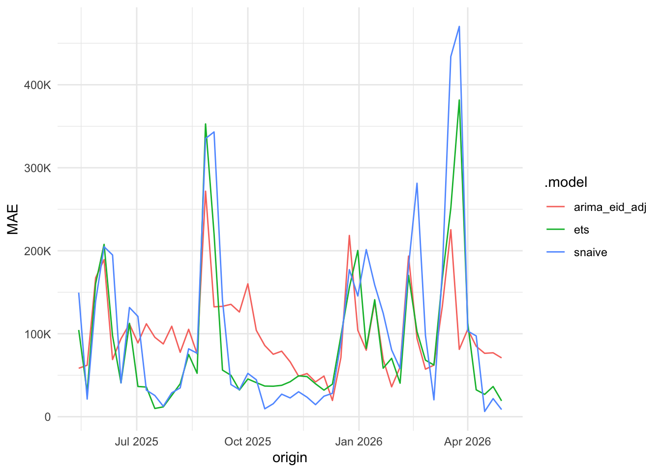
Both ETS and SARIMA model have less than 1 MASE, and performs better than the seasonal naive forecast. We see that although ETS have the best MASE, the SARIMA have lower RMSSE. SARIMA having lower RMSSE implies that SARIMA handles spikes in total passengers better than ETS, but having higher MASE means that the model performs worse in general.
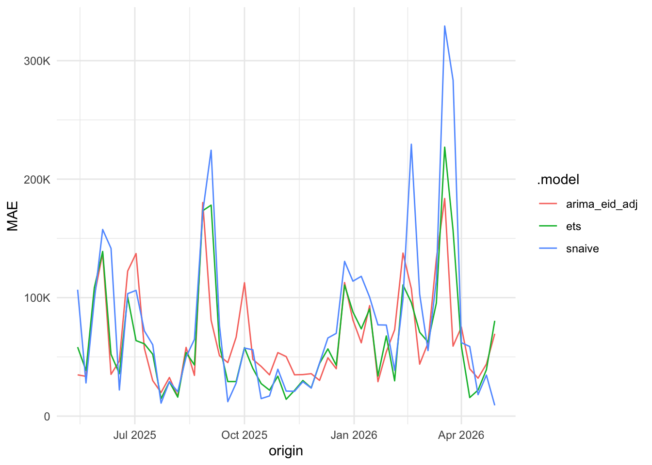
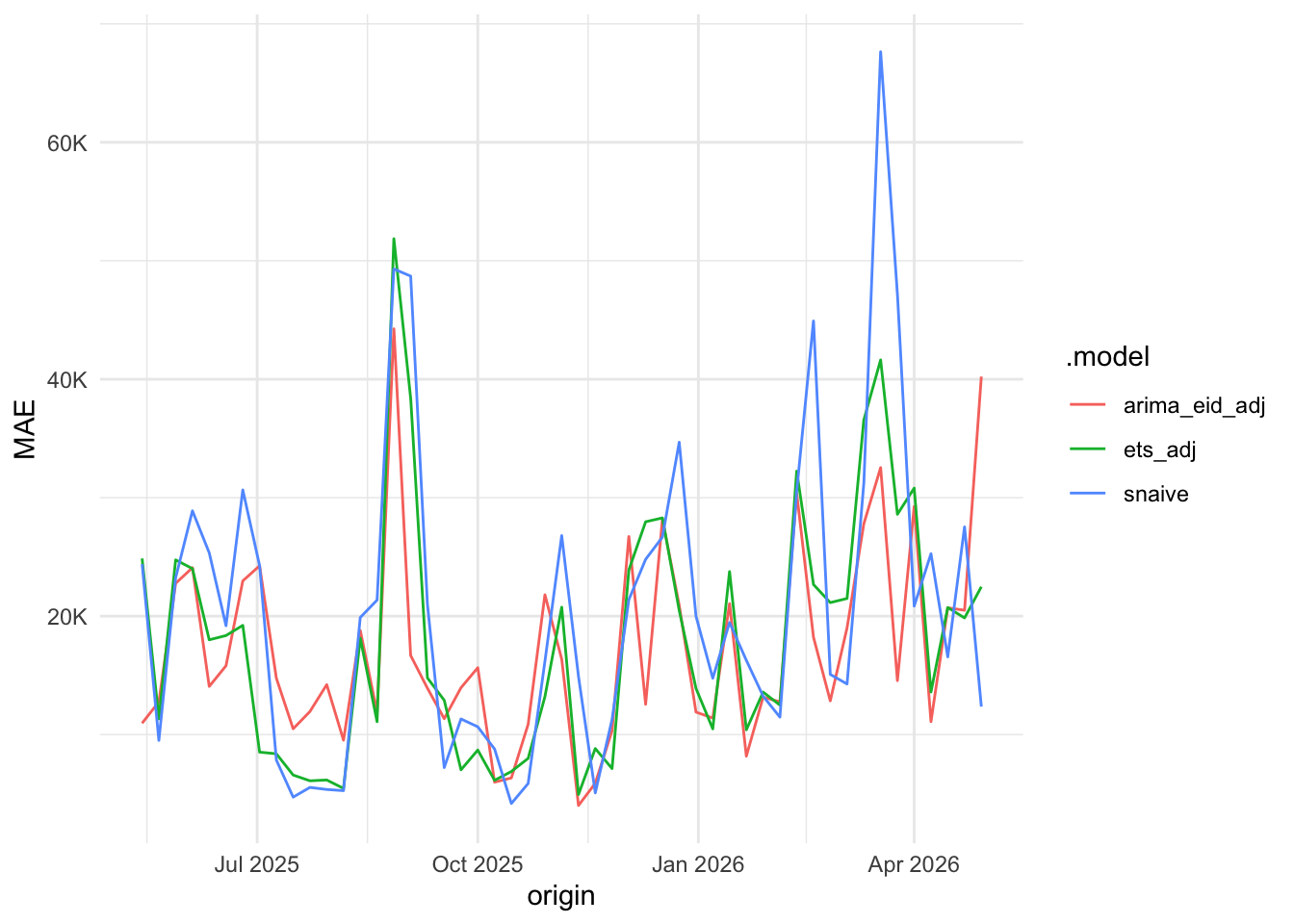
We can see the spike in errors are correlated to the events that we mentioned earlier. Eid, and riot caused some error spikes, but there are other spikes that we did not classify. SARIMA model seem to handle these jumps very well, except at July 2025, but in general when there is no spikes, the ETS model seems to perform better. This seems to be the trade-off that we have right now.
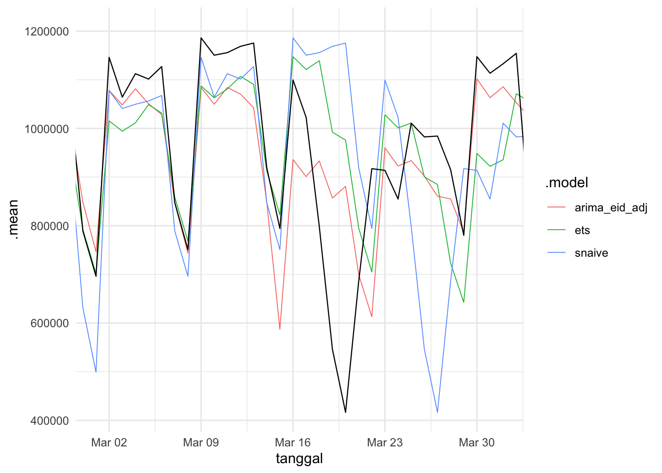
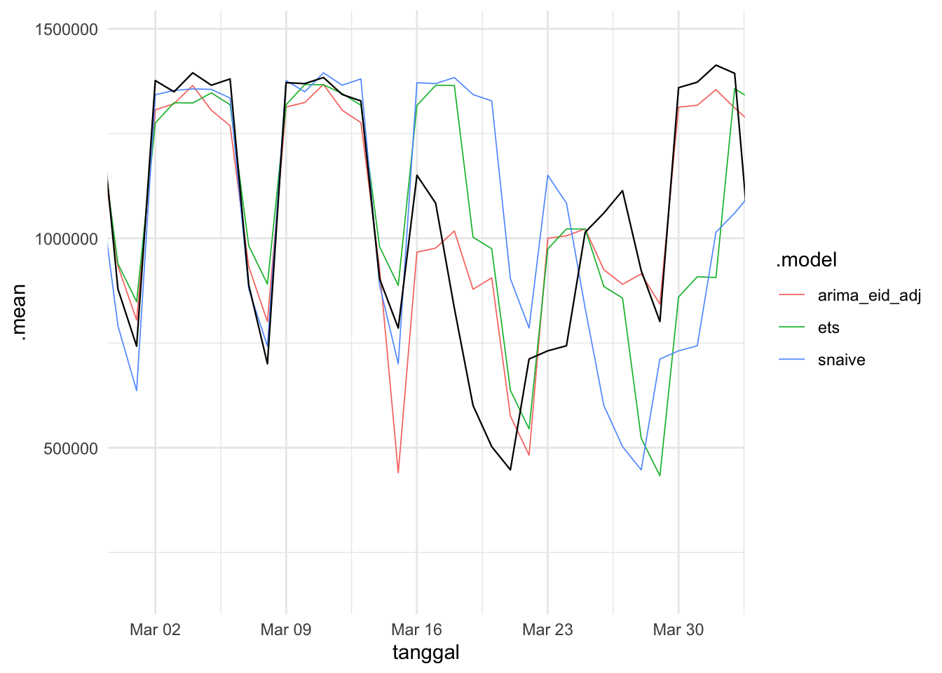
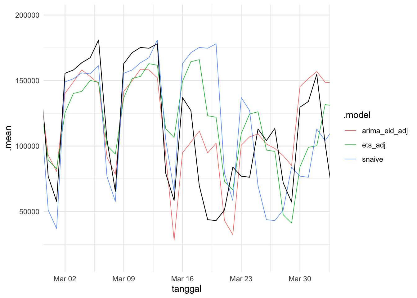
It looks like for the most part, the model underestimates the total passengers compared to the true data. Random dips in total passengers probably played a part in driving the prediction down.
The only model that have Eid as a regressor did adjust for Eid (at 15 March 2026 - 27 March 2026). It didn’t look good at the beginning, but fits better at the later half of the holiday. Do keep in mind that we only have 2 Eid in this case as the training set.
We have the same ETS as KRL, but we have a stronger alpha and a much weaker gamma compared to ETS model for KRL. So, stronger contribution from previous value and much weaker contribution from the last period value.
Already a much different model with 4 order of moving average. The coefficients seems pretty significant too from a first glance. The model seems to have strong reliance on past white noises and no contirbution from the past value are needed except for seasonal differencing.
A very different components from the model without Eid regressor. Now, we have 2 order of autoregressive coefficients, and the second order looks insignificant. This begs some attempts at different parameters manually. It seems that during Eid, according to the is_eid coefficient, the total passengers on average drops by 344K with 45K standard error. A lot more compared to KRL.
The general idea is the same as KRL. But this time, ETS and SARIMA overestimations are more severe. The fluctuations also looks more wild for SNAIVE. Naturally, all models are not considered white noise from the residuals check, but let us see the ljung-box test.
fits_tj %>%augment() %>%filter(.model =="arima_eid_adj") %>%features(.innov, ljung_box, lag =14, dof =2)
Surprisingly, SARIMA model still manages to fail rejecting the null hypothesis while ETS and SNAIVE still rejects. Meaning, the ljung-box test for SARIMA residuals failed to reject that it is white noise with 95% confidence. Same conclusion as KRL model.
The ETS model performs very similarly to KRL model. But the SARIMA model, in general worse MASE compared to both ETS and better RMSSE compared to both ETS.
We can see here that SARIMA model seems to carries the effect from the spike and doesn’t recover quick enough and affects the MAE greatly. It makes sense considering that the non-seasonal component is an AR component. However, as seen during 2026 Eid, the SARIMA handles the change much better compared to the other models, which again, the trade-off that was mentioned.
The SARIMA immediately followed the dip from the data due to the information from the regressor, while the other two are quite late at following the pattern because they did not have that information.
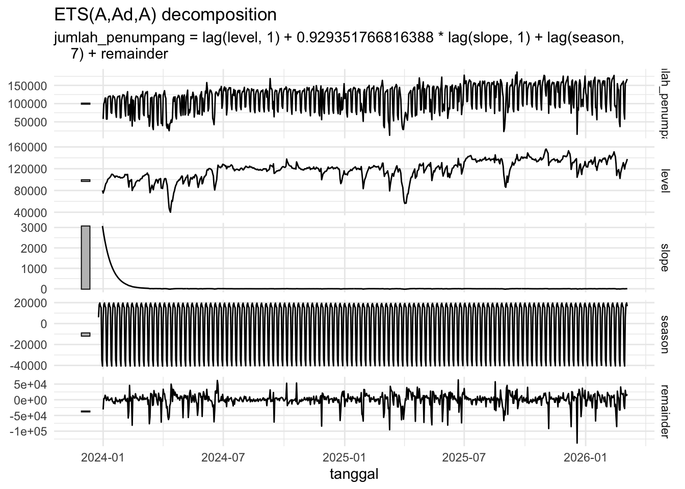
Now the ETS looks different. We have “Ad” for trend which means additive damped. The additive parameter for trend is denoted by beta, which is really weak in this case which affects current trend. While the damping parameter is denoted by phi, which is very high and close to a linear trend. In other words, the trend only happens for a very short time. It is possible that we can ignore this and have the trend be null instead.
Other than that, we have low alpha and very low gamma, similar to KRL model.
We see that the moving average coefficient significance is dwindling due to the standard error increasing. We could apply the same treatment, since if we do \[
-0.1711 \pm 1.96 (0.1204)
\] The confidence interval which is \((-0.407, 0.0649)\) includes zero.
AICc barely affected, but we get to remove a coefficient. According to this model, during eid, the average total passengers drops by ~49K with 5K error.
Both SNAIVE and ETS residuals are quite consistent throughout the transportation methods. However, for SARIMA here, the ACF lines did not cross the blue line, which indicates that the residuals are white noise.
fits_mrt %>%augment() %>%filter(.model =="arima_eid_adj") %>%features(.innov, ljung_box, lag =14, dof =2)
Again, only SARIMA failed to reject the null hypothesis. Also, since there is not much different between ETS and ETS without trend component, we will use ETS without trend as it is simpler, and it is correct to use according to the interpretation of the components.
We can see that SARIMA and ETS MAE overlaps pretty often except during events. A reason for ETS performing worse in MAE might be because of the total passengers being low for MRT.
Same insight, SARIMA follows the event according to the specified date, and ETS followed it after the event.
Conclusion
We can conclude that for KRL and TRANSJAKARTA, there are two possible best models depending on the purpose of the forecast. The ETS model achieves the best MASE (0.802 and 0.817), while the SARIMA model has the best RMSSE (0.722 and 0.690). The ETS model performs the best when forecasting the typical week, while the SARIMA model handles known events better due to the Eid regressor term. For MRT however, the SARIMA model wins in both MASE (0.902) and RMSSE (0.789) so there is no trade-off here.
The main thing that differentiates the ETS model and SARIMA model, aside from the model structure, is the regressor term that we added. It allows the SARIMA model to follow the change that happens during the event immediately, instead of adjusting after the event happened like the ETS model did.
However, in this dataset, the training data only has two Eid so the result might not be optimal. Not to mention, there are one-offs that happened, the August 2025 riot, the November 2024 election holiday (should not be one-offs but with this dataset, they are) and data inconsistencies around Nataru that we had to impute against the BPS data so it only approximates the daily total passengers shape. With a cleaner data around Nataru and more data, Nataru might be added as a regressor term for SARIMA which might change the model performance as well.