import pandas as pdfrom copy import deepcopyimport warningsimport numpy as npimport seaborn as snsimport matplotlib.pyplot as pltfrom matplotlib import MatplotlibDeprecationWarningimport matplotlib.patches as patchesimport randomfrom sklearn.metrics import confusion_matrix from sklearn.model_selection import KFoldfrom sklearn.pipeline import Pipelinefrom pygam import LogisticGAM, f, sfrom sklearn.preprocessing import StandardScalerfrom sklearn.tree import DecisionTreeClassifierfrom sklearn.linear_model import LogisticRegression from sklearn.linear_model import LogisticRegressionCV from sklearn.model_selection import GridSearchCVfrom sklearn.neighbors import KNeighborsClassifierfrom sklearn.svm import SVCfrom sklearn.ensemble import GradientBoostingClassifierfrom sklearn.ensemble import RandomForestClassifierfrom statsmodels.stats.outliers_influence import variance_inflation_factorrandom.seed(42)sns.set_theme(style="whitegrid", palette="pastel", rc={"figure.dpi": 150,"axes.spines.right": False, "axes.spines.top": False, })def save_fig(fig, name): fig.savefig(f"figures/{name}.png", dpi=150)# The boxplot for seaborn likes to spits out PendingDeprecationWarning and I could not figure it out. So I just disable the warning.warnings.filterwarnings("ignore", category=PendingDeprecationWarning)warnings.filterwarnings("ignore", category=MatplotlibDeprecationWarning)
Dataset
This data is gathered from a private hospital in Indonesia. It contains blood test result and the patient treatment given after the blood test. The dataset can be downloaded from here
First, take a glimpse at the dataset to check for irregularities and learn about the features.
Code
df = pd.read_csv("data/data-ori.csv")df
HAEMATOCRIT
HAEMOGLOBINS
ERYTHROCYTE
LEUCOCYTE
THROMBOCYTE
MCH
MCHC
MCV
AGE
SEX
SOURCE
0
35.1
11.8
4.65
6.3
310
25.4
33.6
75.5
1
F
out
1
43.5
14.8
5.39
12.7
334
27.5
34.0
80.7
1
F
out
2
33.5
11.3
4.74
13.2
305
23.8
33.7
70.7
1
F
out
3
39.1
13.7
4.98
10.5
366
27.5
35.0
78.5
1
F
out
4
30.9
9.9
4.23
22.1
333
23.4
32.0
73.0
1
M
out
...
...
...
...
...
...
...
...
...
...
...
...
4407
32.8
10.4
3.49
8.1
72
29.8
31.7
94.0
92
F
in
4408
33.7
10.8
3.67
6.7
70
29.4
32.0
91.8
92
F
in
4409
33.2
11.2
3.47
7.2
235
32.3
33.7
95.7
93
F
out
4410
31.5
10.4
3.15
9.1
187
33.0
33.0
100.0
98
F
in
4411
33.5
10.9
3.44
5.8
275
31.7
32.5
97.4
99
F
out
4412 rows × 11 columns
Code
df.describe()
HAEMATOCRIT
HAEMOGLOBINS
ERYTHROCYTE
LEUCOCYTE
THROMBOCYTE
MCH
MCHC
MCV
AGE
count
4412.000000
4412.000000
4412.000000
4412.000000
4412.000000
4412.000000
4412.000000
4412.000000
4412.000000
mean
38.197688
12.741727
4.541260
8.718608
257.524479
28.234701
33.343042
84.612942
46.626473
std
5.974784
2.079903
0.784091
5.049041
113.972365
2.672639
1.228664
6.859101
21.731218
min
13.700000
3.800000
1.480000
1.100000
8.000000
14.900000
26.000000
54.000000
1.000000
25%
34.375000
11.400000
4.040000
5.675000
188.000000
27.200000
32.700000
81.500000
29.000000
50%
38.600000
12.900000
4.570000
7.600000
256.000000
28.700000
33.400000
85.400000
47.000000
75%
42.500000
14.200000
5.050000
10.300000
321.000000
29.800000
34.100000
88.700000
64.000000
max
69.000000
18.900000
7.860000
76.600000
1183.000000
40.800000
39.000000
115.600000
99.000000
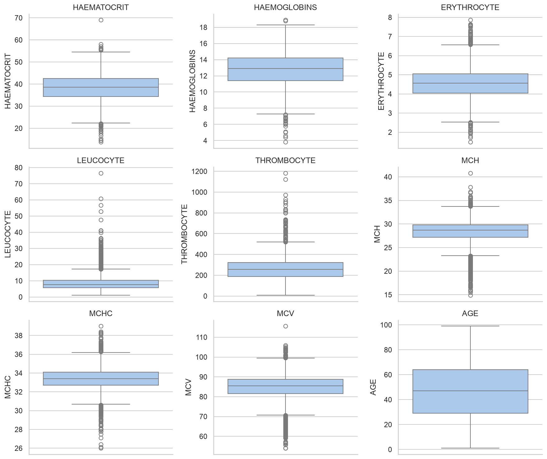
Interesting that the minimum age is 1 and the maximum is 99, seems convenient. It is also interesting that some of the maximum values are insanely far from the mean.
Let us do some one factor encoding for the output (SOURCE) and (SEX). - 1 For Male - 1 For in-care
Code
df['SEX'] = [1if i =='M'else0for i in df['SEX'] ]df['SOURCE'] = [1if i =='in'else0for i in df['SOURCE']]
It seems that there is a slight class imbalance, where patients who are given out of care treatments are \(\approx 60\%\) of the data
Outliers
Code
numeric_feat = [i for i in df.columns if i notin ["SEX", "SOURCE"]]fig, axes = plt.subplots(3, 3, figsize=(12, 10))for ax, col inzip(axes.flatten(), numeric_feat): sns.boxplot(df[col], ax=ax) ax.set_title(col)plt.tight_layout()
Consistent with our finding in df.describe() earlier. There are no negatives so the outliers will not be removed. Especially since I do not know whether the outliers usually happens with really sick people or not. (Simply put, no domain knowledge)
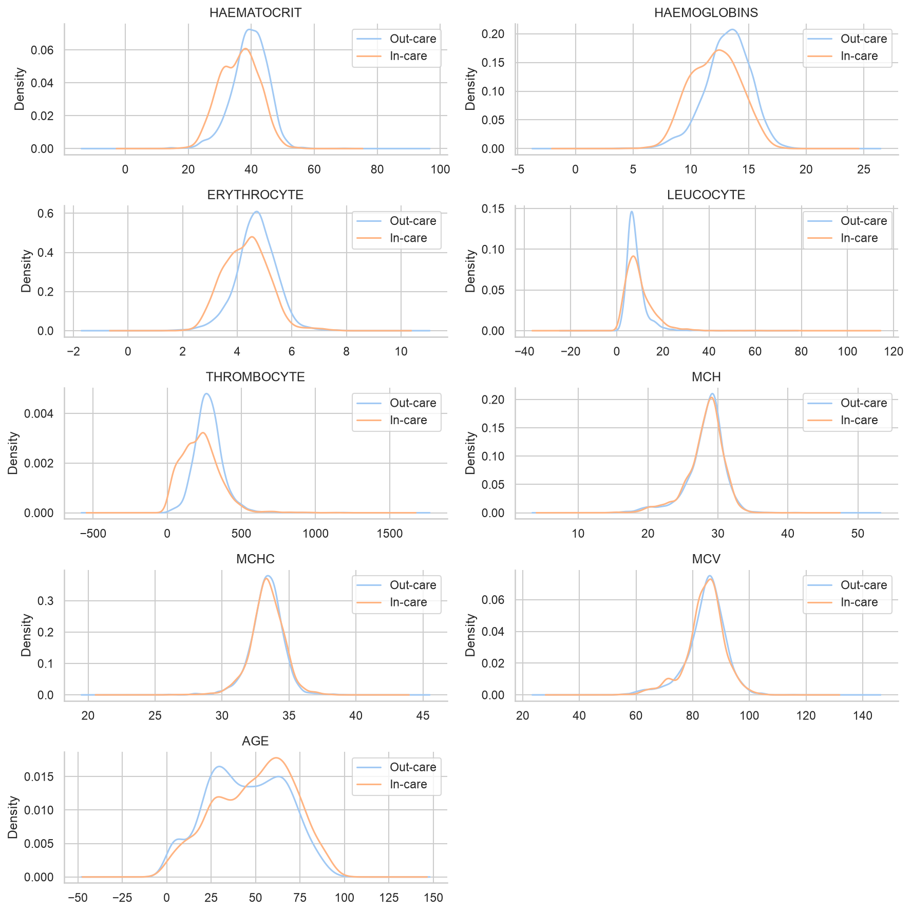
Seems normal, no extreme skewness or anything to worry about. None of the data actually went into the negative, so it must be from the plot. Regarding the densities difference, both classes seem to overlap heavily and there are barely any distinction between the two. Therefore, the expectation of the models that we are about to do should be low.
Code
df['SEX'].value_counts()
SEX
1    2290
0    2122
Name: count, dtype: int64
Looks really balanced for the only categorical predictor we have.
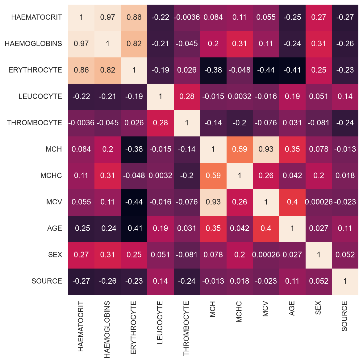
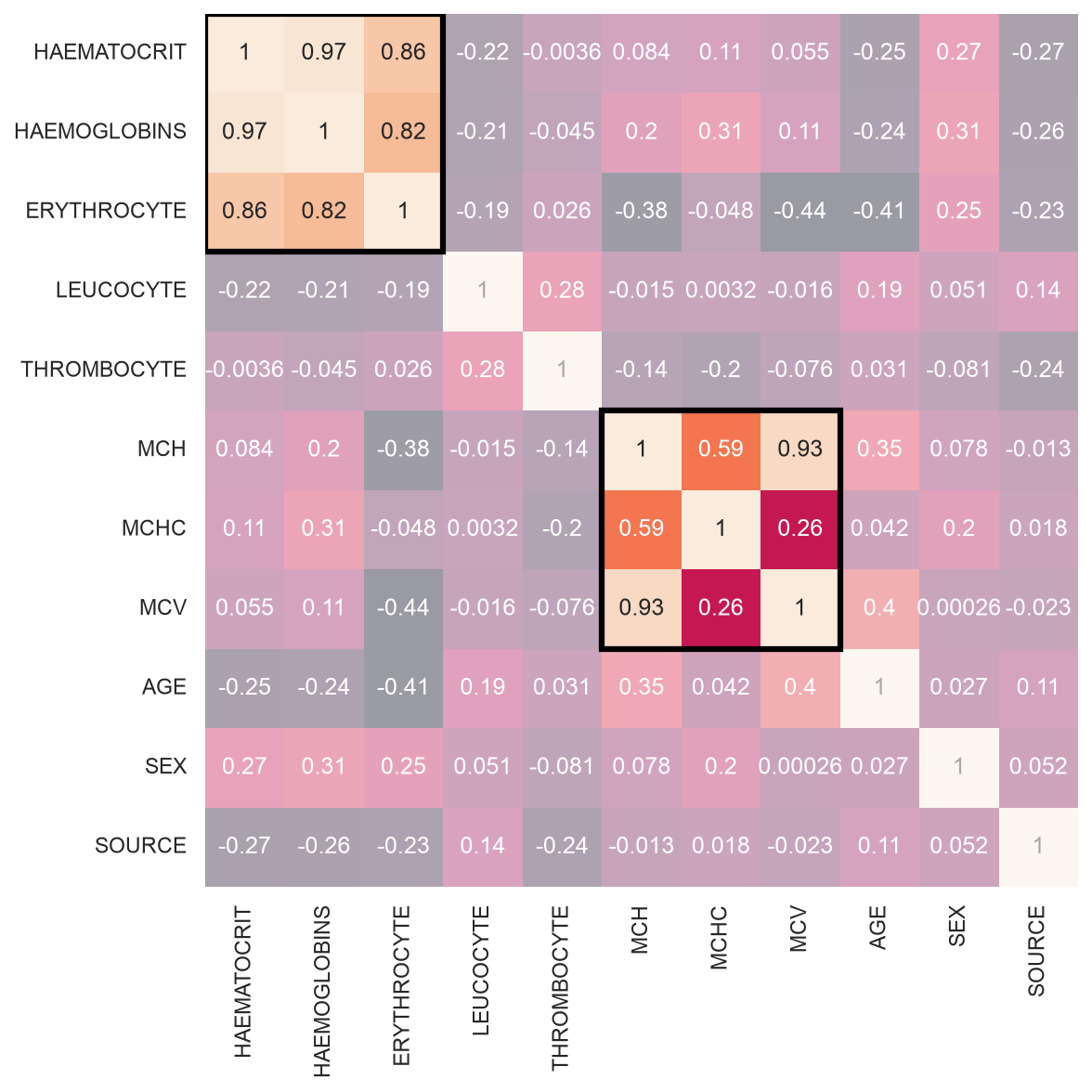
# For highlightingfig, ax = plt.subplots(figsize=(8,8))sns.heatmap(df.corr(), annot=True, ax=ax, cbar=False)n =len(df.columns)veil =dict(facecolor="white", alpha=0.6, edgecolor="none", zorder=3)ax.add_patch(patches.Rectangle((3, 0), n-3, n-6, **veil)) # right of 1st clusterax.add_patch(patches.Rectangle((8, 5), n-8, n-5, **veil)) # right of 2nd clusterax.add_patch(patches.Rectangle((3, 5), 2, 3, **veil)) # left of 2nd clusterax.add_patch(patches.Rectangle((0, 3), 3, n-3, **veil)) # below 1st clusterax.add_patch(patches.Rectangle((3, 8), 5, n-3, **veil)) # below 2nd cluster# ax.add_patch(patches.Rectangle((5, 0), 3, 5, **veil)) # above block# Borderax.add_patch(patches.Rectangle((0, 0), 3, 3, fill=False, edgecolor="black", lw=3, zorder=4)) # First clusterax.add_patch(patches.Rectangle((5, 5), 3, 3, fill=False, edgecolor="black", lw=3, zorder=4)) # Second clusterplt.tight_layout()save_fig(fig, "Corr12")plt.show()
There are no strong correlation between any of the predictors and the target variable (SOURCE). But, we can see that there are some multicolinearity going on with the predictors. For example, HAEMOGLOBINS have a very strong correlation with HAEMATOCRIT. Which makes sense, because by definition, HAEMOGLOBINS are a protein that is contained in red blood cells while HAEMATOCRIT are volume of red blood cells relative to total blood cells.
Variance Inflation Factor (VIF)
Because we have multicollinearity, and I do not have medical background to justify direct feature elimination, I will perform iterative feature selection using VIF by eliminating features that have VIF > 10.
Code
to_remove = ["SOURCE"]max_vif =11while max_vif >10: vif_data = pd.DataFrame() feature_col = [features for features in df.columns if features notin to_remove] vif_data["feature"] = feature_col vif_data["VIF"] = [variance_inflation_factor(df[feature_col].values, i)for i inrange(len(feature_col))]print(vif_data) max_vif = vif_data['VIF'].max() highest_vif = vif_data.iloc[vif_data['VIF'].idxmax()]['feature']if max_vif <=10:breakprint("Next Remove:", highest_vif, "VIF:",max_vif, "\n") to_remove.append(highest_vif)
The predictors distributions looks pretty normal and there are no imbalance within the categorical predictor.
There is a slight class imbalance on the target variable (60/40), but should not pose a problem and there will be no action taken.
There are a lot of outliers but none of them are in the negatives (which I know is impossible), but since I do not know whether the outliers are considered normal for sick people, there will be no action taken.
There are some strong multicollinearity going on with (HAEMATOCRIT - HAEMOGLOBINS - ERYTHROCYTE), and (MCH - MCV).
There are some moderate multicollinearity going on with (MCH- MCHC).
The multicollinearity predictors will be reduced for some models but, the full model will be shown as well.
After feature selection, we are left with 5 features, which are - ERYTHROCYTE - LEUCOCYTE - THROMBOCYTE - AGE - SEX
Modelling Functions
Added as extended analysis after the course. Mostly refactoring to keep things clean. Also, I’ve added scaling cost that punishes false negatives and lower the threshold for every model to predict for In-Care treatment.
Code
def kfold_data(df, n_splits):''' Split data using K-fold cross validation. ''' kf = KFold(n_splits= n_splits) train_indexes = [] test_indexes = []for train_index, test_index in kf.split(df): train_indexes.append(train_index) test_indexes.append(test_index)return train_indexes, test_indexesdef get_metrics(costs, pred_proba, y_test):''' Compute multiple costs for misclassification rate. ''' result = []for i in costs: weighted_pred = []for j in pred_proba: weighted_pred.append(np.argmax(j * [1, i])) cf = confusion_matrix(y_test, np.array(weighted_pred)) TN, FP = cf[0][0], cf[0][1] FN, TP = cf[1][0], cf[1][1] expected_cost = (i * FN + FP) / np.sum(cf) sensitivity = TP / (TP + FN) specificity = TN / (TN + FP) result.append([i, expected_cost, sensitivity, specificity])# Returns a listreturn resultdef get_gam_metrics(costs, y_pred, y_test): result = []for i in costs: threshold =1/ (1+i) weighted_pred = (y_pred > threshold).astype(int) cf = confusion_matrix(y_test, np.array(weighted_pred)) TN, FP = cf[0][0], cf[0][1] FN, TP = cf[1][0], cf[1][1] expected_cost = (i * FN + FP) / np.sum(cf) sensitivity = TP / (TP + FN) specificity = TN / (TN + FP) result.append([i, expected_cost, sensitivity, specificity])return resultdef cv_predict(df, model, model_name, train_indexes, test_indexes, to_remove, grid_search):''' Use K-fold cross validation to predict and log results. ''' models = [] results = []for fold inrange(len(train_indexes)):# Dataset split X_train = df[[i for i in df.columns if i notin to_remove]].iloc[train_indexes[fold]] Y_train = df['SOURCE'].iloc[train_indexes[fold]] x_test = df[[i for i in df.columns if i notin to_remove]].iloc[test_indexes[fold]] y_test = df['SOURCE'].iloc[test_indexes[fold]]if grid_search:# Train model.fit(X_train, Y_train) models.append(deepcopy(model))# models.append(search_model.cv_results_['mean_test_score'])# Test pred_proba = model.best_estimator_.predict_proba(x_test)else:# Train model.fit(X_train, Y_train) models.append(deepcopy(model))# Test pred_proba = model.predict_proba(x_test)# Get metrics metrics = get_metrics([1, 3], pred_proba, y_test)for c inrange(len(metrics)): results.append( [model_name, fold] + metrics[c])# Returns list of confusion matrices?, list of model objects, and dfreturn models, pd.DataFrame(results, columns=['model_name', 'fold', 'cost', 'expected_cost', 'sensitivity', 'specificity'])def gam_predict(df, model_name, train_indexes, test_indexes, is_reduced): models = [] results = []for fold inrange(len(train_indexes)): X_train = df[[i for i in df.columns if i !="SOURCE"]].iloc[train_indexes[fold]] Y_train = df['SOURCE'].iloc[train_indexes[fold]] x_test = df[[i for i in df.columns if i !="SOURCE"]].iloc[test_indexes[fold]] y_test = df['SOURCE'].iloc[test_indexes[fold]]if is_reduced: x_test = x_test[[i for i in df.columns if i in ['ERYTHROCYTE', 'LEUCOCYTE', 'THROMBOCYTE', 'AGE', 'SEX']]] X_train_gam = np.column_stack([X_train['ERYTHROCYTE'], X_train['LEUCOCYTE'], X_train['THROMBOCYTE'], X_train['AGE'], pd.Categorical(X_train['SEX']).codes]) gam = LogisticGAM(s(0) + s(1) + s(2) + s(3) + f(4), verbose=False).gridsearch( X_train_gam, pd.Categorical(Y_train).codes, lam= [np.logspace(-2, 2, 3)]*5)else: X_train_gam = np.column_stack([X_train['HAEMATOCRIT'], X_train['HAEMOGLOBINS'], X_train['ERYTHROCYTE'], X_train['LEUCOCYTE'], X_train['THROMBOCYTE'], X_train['MCH'], X_train['MCHC'], X_train['MCV'], X_train['AGE'], pd.Categorical(X_train['SEX']).codes]) gam = LogisticGAM(s(0) + s(1) + s(2) + s(3) + s(4) + s(5) + s(6) + s(7) + s(8) + f(9), verbose=False).gridsearch( X_train_gam, pd.Categorical(Y_train).codes, lam=np.logspace(-3, 3, 11)) models.append(deepcopy(gam)) pred_proba = gam.predict_proba(x_test) metrics = get_gam_metrics([1, 3], pred_proba, y_test)for c inrange(len(metrics)): results.append( [model_name, fold] + metrics[c])return models, pd.DataFrame(results, columns=['model_name', 'fold', 'cost', 'expected_cost', 'sensitivity', 'specificity'])def log_result(models, res, temps): models.append(temps[0]) res = pd.concat([res, temps[1]]).reset_index(drop=True)return models, resmodels, res = [], pd.DataFrame(columns=['model_name', 'fold', 'cost', 'expected_cost', 'sensitivity', 'specificity'])train_indexes, test_indexes = kfold_data(df, 5)
Logistic regression
First, I will try the simplest classification model. Additionally, I will use Ridge and Lasso penalties to help with the multicollinearity and give weight to features.
For cleanliness, I will ignore FutureWarning that basically states a new way to set a penalty for this model.
Next, is a non-parametric model. Though, from the distribution plot earlier, I doubt the model will perform well since there are barely any distinction between the treatment groups.
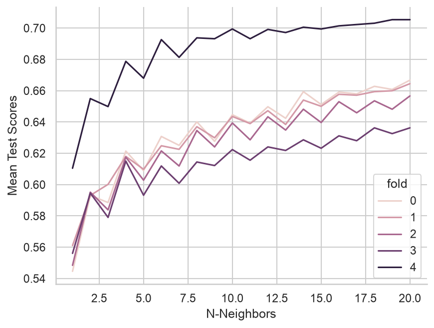
sns.lineplot(data=k_cv, x='n_neighbors', y='mean_test_scores', hue='fold')plt.ylabel("Mean Test Scores")plt.xlabel("N-Neighbors")plt.show()
It seems that as n_neighbors increases, the scores also increases. There might be not a meaningful clusters so this model might not help since if k increases towards the entire data, then the ‘nearest neighbors’ concept is discarded.
Generalized additive models
Due to multicollinearity, the model will spits out a bunch of warning during fitting. This also happens to reduced model where I removed the variables with high correlation with each other. But, it only happens during some section of the gridsearch for the penalty term, so it might be caused by that for the reduced model.
LogisticGAM
=============================================== ==========================================================
Distribution:                      BinomialDist Effective DoF:                                     40.2517
Link Function:                        LogitLink Log Likelihood:                                 -1879.4705
Number of Samples:                         3529 AIC:                                             3839.4443
                                                AICc:                                            3840.4441
                                                UBRE:                                               3.0971
                                                Scale:                                                 1.0
                                                Pseudo R-Squared:                                   0.2164
==========================================================================================================
Feature Function                  Lambda               Rank         EDoF         P > x        Sig. Code
================================= ==================== ============ ============ ============ ============
s(0)                              [15.8489]            20           6.3          1.64e-02     *
s(1)                              [15.8489]            20           3.9          3.09e-04     ***
s(2)                              [15.8489]            20           4.6          3.27e-01
s(3)                              [15.8489]            20           4.0          0.00e+00     ***
s(4)                              [15.8489]            20           4.8          0.00e+00     ***
s(5)                              [15.8489]            20           4.0          3.91e-03     **
s(6)                              [15.8489]            20           3.6          4.83e-04     ***
s(7)                              [15.8489]            20           2.3          1.11e-02     *
s(8)                              [15.8489]            20           5.9          9.89e-04     ***
f(9)                              [15.8489]            2            0.9          4.95e-12     ***
intercept                                              1            0.0          2.99e-02     *
==========================================================================================================
Significance codes:  0 '***' 0.001 '**' 0.01 '*' 0.05 '.' 0.1 ' ' 1

WARNING: Fitting splines and a linear function to a feature introduces a model identifiability problem
         which can cause p-values to appear significant when they are not.

WARNING: p-values calculated in this manner behave correctly for un-penalized models or models with
         known smoothing parameters, but when smoothing parameters have been estimated, the p-values
         are typically lower than they should be, meaning that the tests reject the null too readily.
There are a lot of errors, since it uses Iterative Reweighted Least Squares, it might be because of multicollinearity. Additionally, the lambda are all the same which means, every features are penalized the same amount. This is not an optimal result but tuning the penalties will take a long time.
Reduced Model
I used the result of feature selection that was performed earlier using VIF.
LogisticGAM
=============================================== ==========================================================
Distribution:                      BinomialDist Effective DoF:                                     29.6974
Link Function:                        LogitLink Log Likelihood:                                   -1952.92
Number of Samples:                         3529 AIC:                                             3965.2349
                                                AICc:                                            3965.7914
                                                UBRE:                                               3.1303
                                                Scale:                                                 1.0
                                                Pseudo R-Squared:                                   0.1857
==========================================================================================================
Feature Function                  Lambda               Rank         EDoF         P > x        Sig. Code
================================= ==================== ============ ============ ============ ============
s(0)                              [1.]                 20           10.0         0.00e+00     ***
s(1)                              [1.]                 20           6.3          0.00e+00     ***
s(2)                              [1.]                 20           8.4          0.00e+00     ***
s(3)                              [100.]               20           4.1          1.48e-03     **
f(4)                              [1.]                 2            1.0          1.21e-06     ***
intercept                                              1            0.0          6.10e-01
==========================================================================================================
Significance codes:  0 '***' 0.001 '**' 0.01 '*' 0.05 '.' 0.1 ' ' 1

WARNING: Fitting splines and a linear function to a feature introduces a model identifiability problem
         which can cause p-values to appear significant when they are not.

WARNING: p-values calculated in this manner behave correctly for un-penalized models or models with
         known smoothing parameters, but when smoothing parameters have been estimated, the p-values
         are typically lower than they should be, meaning that the tests reject the null too readily.
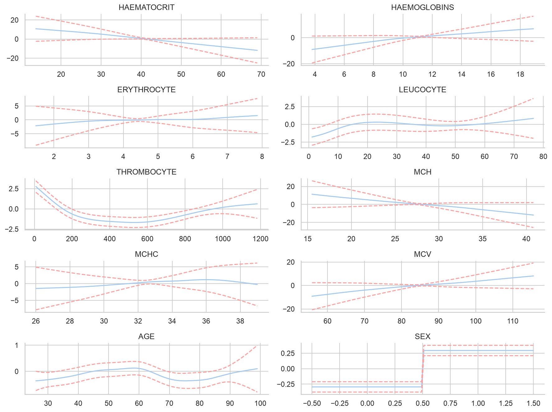
We can see how the multicollinearity affect each features. It is expected that the full model will have large confidence bands for features that are affected by multicollinearity.
Code
fig, axs = plt.subplots(5, 2, figsize=(12, 9))titles = df[[i for i in df.columns if i !="SOURCE"]].columnsfor i, ax inenumerate(axs.flat): XX = gam_models[0].generate_X_grid(term=i) pdep, confi = gam_models[0].partial_dependence(term=i, width=0.95) sns.lineplot(x=XX[:, i], y=pdep, ax=ax) sns.lineplot(x=XX[:, i], y=confi[:, 1], c="r", ls="--", ax=ax) sns.lineplot(x=XX[:, i], y=confi[:, 0], c="r", ls="--", ax=ax) ax.set_title(titles[i])fig.tight_layout()save_fig(fig, "PD_F")plt.show()
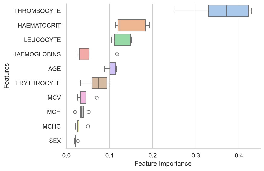
It seems that these features that are affected by multicollinearity are also deemed important since most of them have very high importance relative to other features.
By reducing the model based on feature selection, I expect tighter confidence bands. While I do not have medical background, I assume that these metrics are there for a reason despite the strong correlation. Therefore, the model might lose some predictive ability from this reduction but I can get a much clearer interpretation of each features that are not correlated.
Code
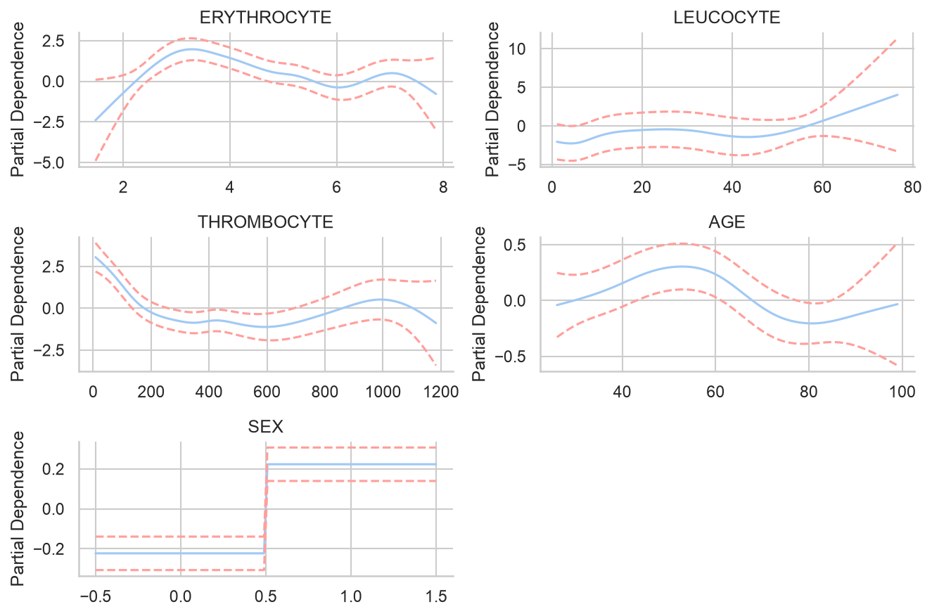
fig, axs = plt.subplots(3, 2, figsize=(9, 6))titles = df[[i for i in df.columns if i notin to_remove]].columnsfor i, ax inenumerate(axs.flat):if i >=len(titles): fig.delaxes(ax)break XX = gamr_models[0].generate_X_grid(term=i) pdep, confi = gamr_models[0].partial_dependence(term=i, width=0.95) sns.lineplot(x=XX[:, i], y=pdep, ax=ax) sns.lineplot(x=XX[:, i], y=confi[:, 1], c="r", ls="--", ax=ax) sns.lineplot(x=XX[:, i], y=confi[:, 0], c="r", ls="--", ax=ax) ax.set_title(titles[i]) ax.set_ylabel('Partial Dependence')fig.tight_layout()save_fig(fig, "PD_R")plt.show()
There are widening of confidence bands at the edge, presumably due to the lack of data at that points.
These partial dependence does not seem to have linear relationships with the treatment choice, which is to be expected. - It seems that the patient that have ERYTHROCYTE between 2 until 6 are more likely to be admitted to In-care treatment. - Patients that have LEUCOCYTE more than ~40, are more likely to be given In-care treatment. - Patients that have THROMBOCYTE between 0 and 200, are also more likely to be given In-care treatment. The same applies for range between ~800 and ~1100 - Interestingly, patients that are aged between ~40 and ~60 are more likely to be given In-care treatment. I would expect the reverse of this. But again, the partial dependence looks relatively weak. - Male patients are more likely to be given In-care treatment though the partial dependence have the smallest scale among the other features.
Decision trees and ensemble methods
Then, we use decision trees which is probably going to do bad since it is a very simple model and quickly move on to ensemble methods, particularly random forest and gradient boost. - Because the random forest uses deep trees, it will have high variance and tries to reduce it by averaging a lot of trees - The gradient boost start with a shallow tree and sequentially fits the residuals, meaning it will initially start with high bias and reduce it as more trees fitted.
Decision Tree
Code
dtree = DecisionTreeClassifier(random_state=42)parameters_dtrees = {'max_depth': [i for i inrange(1, 10, 1)]}gs_dtrees = GridSearchCV(dtree, parameters_dtrees)models, res = log_result(models, res, cv_predict(df, gs_dtrees, 'DT', train_indexes, test_indexes, ["SOURCE"], True))
Random Forest
Code
rforest = RandomForestClassifier(random_state=42)parameters_rforests = {"n_estimators":[i for i inrange(20, 100, 20)], "max_features": ['sqrt', 'log2', 5, 7, 9]}gs_rforest = GridSearchCV(rforest, parameters_rforests)models, res = log_result(models, res, cv_predict(df, gs_rforest, 'RF', train_indexes, test_indexes, ["SOURCE"], True))
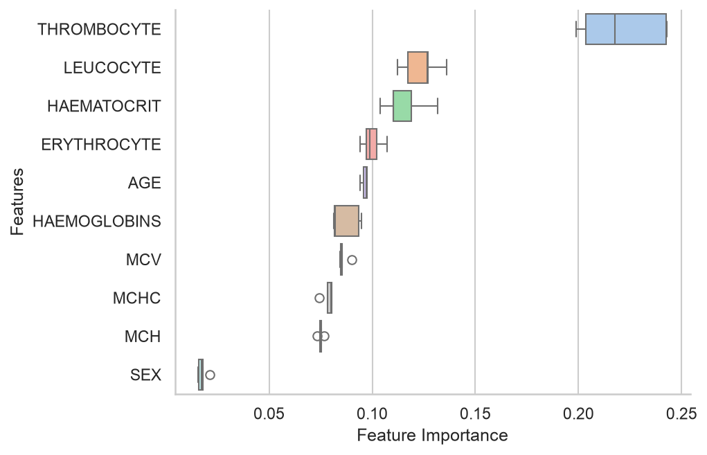
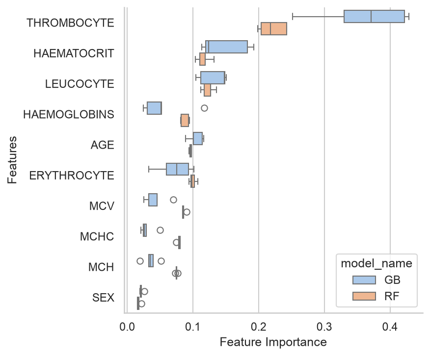
The ensemble methods provide feature importance and from it, I can see which feature are deemed important by the model.
Code
rf_features = {f : [] for f in df.columns if f !="SOURCE"}for i in models[-1]:for importance, names inzip(i.best_estimator_.feature_importances_, i.best_estimator_.feature_names_in_): rf_features[names].append(importance)
gb_features = {f : [] for f in df.columns if f !="SOURCE"}for i in models[-1]:for importance, names inzip(i.best_estimator_.feature_importances_, i.best_estimator_.feature_names_in_): gb_features[names].append(importance)
Here, the comparison of importance can be seen between Gradient boost model which is more aggressive, and Random forest.
Support vector machine
Finally, I will try SVM, but unfortunately, this model requires a lot of hyperparameter tuning and my machine can not support it. Hence, the result might be sub optimal.
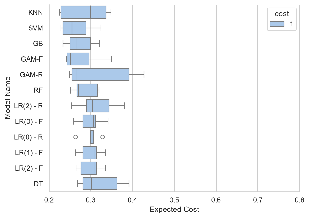
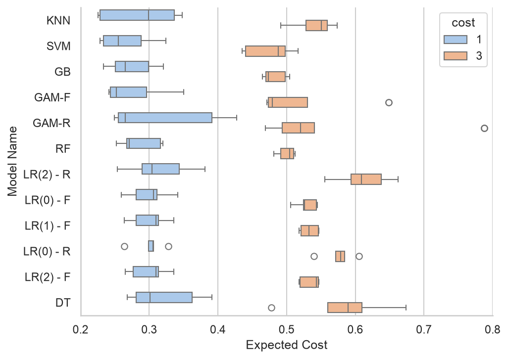
If we set the cost to 1, the metric will be equal to misclassification rate. While the KNN model have the lowest misclassification rate in one of the fold, the result varies too much as indicated by the wide box. To me, the best results are SVM, Gradient Boost, and GAM-F.
But, the mislcassification rate alone does not tell the whole story. Here, it is explained that most of the model have low sensitivity, which means it misses a lot of patients that were supposed to be given In-Care treatment. This is really bad in this context, because missing an In-Care treatment can be dangerous for patients.
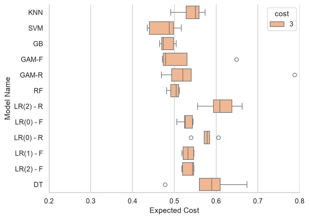
This is the result where the cost of getting a False Negative (Missed an In-care treatment) is tripled and the models are more likely to give In-Care treatment. The three best models perform similarly, which are SVM, Gradient Boost, and RF
By increasing the cost of False Negative and reducing the threshold for the model to predict In-Care treatment, there is a massive increase in sensitivity for all models, in exchange for specificity. From the table, we can see the top three model is actually SVM, Gradient Boost, and Random Forest. The Random forest has a much tighter box which helps the mean expected cost. All three perform similarly though.
Prediction wise, SVM have the best performance in both costs. But, do note that SVM model hyperparameter is not optimally tuned and it does takes a long time to train in comparison to all other models. Considering the time and requirements of SVM, I would say that Gradient Boost provides a consistent best prediction amongst all models but also requires a significant training time. With some performance trade off, I can also suggest using GAM-F model for some interpretability. Do note that GAM models required penalties to every features and in this project, it is not fully explored.
It is also important to note that for the ensemble methods, the probability of prediction works differently because of the nature of the model. Random forest model, by definition creates many deep decision trees and averages out the prediciton of every trees. This makes the random forest model lean more towards the center since it averages out the extreme by sheer number of trees. While Boosting model, sequentially create a low depth trees using the errors from previous trees, which pushes the probabilities toward extremes as the number of trees grows. Consequently, this does not align with the whole different threshold for the expected cost that was implemented. For example, when cost = 3, the probability threshold for the model to predict In-Care is 0.25, but as explained earlier, these ensemble methods probabilities are derived from the combination of number of trees and because of that, these models do not fully follow the behavior that I intend to induce by introducing the higher cost.
Regardless of the result, as stated in the beginnning during EDA, the distribution of every features overlaps for both of the treatments and these result are expected.