Go back to write-up

Import Libraries

import pandas as pd
import seaborn as sns
import matplotlib.pyplot as plt
import scipy.stats as stats
import numpy as np
from statsmodels.stats.proportion import proportions_ztest
from statsmodels.stats.power import NormalIndPower
import matplotlib.ticker as ticker
from great_tables import GT, md

Dataset Descriptions

The dataset is from A/B test of a game “Cookie Cats” where they are trying to see what happens when moving the first gate from level 30 to level 40. There are 90189 new players while the test is running. When players first installed the game, they were randomly assigned to either gate 30 or gate 40.

df = pd.read_csv("./data/cookie_cats.csv")
df.head()

	userid	version	sum_gamerounds	retention_1	retention_7
0	116	gate_30	3	False	False
1	337	gate_30	38	True	False
2	377	gate_40	165	True	False
3	483	gate_40	1	False	False
4	488	gate_40	179	True	True

userid: Unique ID for each users
version: Whether users have the gate 30 version or the gate 40 version
sum_gamerounds: Total rounds played in the first 14 days.
retention_1: Whether players came back on the 1st day after install
retention_7: Whether players came back on the 7th day after install

df.info()

<class 'pandas.DataFrame'>
RangeIndex: 90189 entries, 0 to 90188
Data columns (total 5 columns):
 #   Column          Non-Null Count  Dtype
---  ------          --------------  -----
 0   userid          90189 non-null  int64
 1   version         90189 non-null  str  
 2   sum_gamerounds  90189 non-null  int64
 3   retention_1     90189 non-null  bool 
 4   retention_7     90189 non-null  bool 
dtypes: bool(2), int64(2), str(1)
memory usage: 2.2 MB

No missing data spotted.

df.nunique()

userid            90189
version               2
sum_gamerounds      942
retention_1           2
retention_7           2
dtype: int64

df.describe()

	userid	sum_gamerounds
count	9.018900e+04	90189.000000
mean	4.998412e+06	51.872457
std	2.883286e+06	195.050858
min	1.160000e+02	0.000000
25%	2.512230e+06	5.000000
50%	4.995815e+06	16.000000
75%	7.496452e+06	51.000000
max	9.999861e+06	49854.000000

49K sum of gameround is insane. Assuming 1 rounds takes 1 minutes, that means the person spent 49000 minutes in 14 days. 49000 minutes translates to 34 days, which we can safely assume, it is impossible to have this many rounds. We will be removing that data, and filter out total game rounds that exceeds 5000 rounds. 5000 rounds is a bit arbitrary, which according to our assumption translates to 3.5 days. Not that it matters since there are no data in between around 3000 and around 49000.

df_clean = df[df['sum_gamerounds'] < 5000].copy()

“Gate” is defined as a stopping point where player could not progress unless they wait or they pay. The objective for that feature is to prevent players from burning out and dropping the game early.
Retention is defined as player coming back at day n
Game rounds are summed from the first 14 day install.

df_clean['version'].value_counts()

version
gate_40    45489
gate_30    44699
Name: count, dtype: int64

It does not look like we have a clean 50/50. We will be testing this later since uneven splits might introduce some bias.

Assumptions and Unknowns

Assumptions: - “Round” is not the same as “level”, rounds can be defined as attempts

Unknowns: - How would the subsequent gates behave? (This would affec how many game rounds are reasonable within the first 14 days)

EDA

Now, let us remind ourself what the objective of the analysis is. The dataset description says that “examine what happens when the first gate in the game was moved from level 30 to level 40”.

So, the company wants to know, whether moving the first stopping point, would affect the players’ behaviour (retention and rounds played). It is not clear what are the behaviour that the company prefers, so we will inspect both behaviour and provide recommendations.

However, we will be treating retention_7 as our primary metric due to the desirableness of player stickiness in gaming and also supported by sum_gamerounds as our secondary metric.

Explore

ax = sns.ecdfplot(df_clean, x='sum_gamerounds', hue='version', log_scale=True)
ax.xaxis.set_major_formatter(ticker.ScalarFormatter())
plt.show()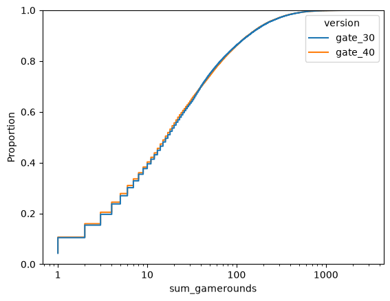

sns.boxplot(df_clean, x='sum_gamerounds', hue='version')
plt.show()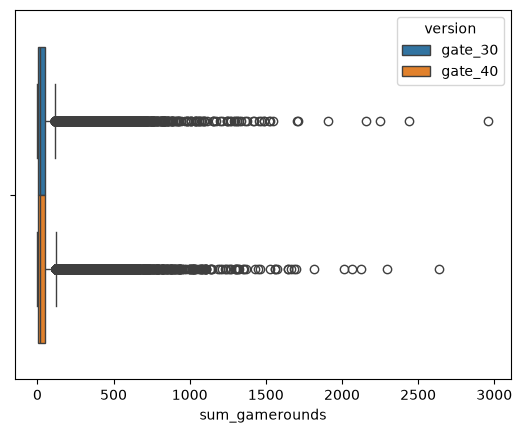

Most players did not play hundreds or thousands of rounds. However, there are some players that played so much more.

Analysis

Is it actually randomized?

Using Pearson’s chi squared goodness of fit for a sample ratio mismatch to test for the 50/50 split. While it is not explicitly stated that the experiment used 50/50, but there is no reason to not assume a 50/50 split.

\(H_0\): No significant difference between the sample and expected ratio

\(H_1\): There is a significant difference between the sample and expected ratio

obs = df['version'].value_counts()
n_total = obs.sum()
expected = [n_total / 2, n_total / 2]

chi2, p_val = stats.chisquare(f_obs=[obs['gate_30'], obs['gate_40']], f_exp=expected)

print(f"chi2 = {chi2:.3f}, p = {p_val:.4f}")

chi2 = 6.902, p = 0.0086

P-value < 0.05, so we reject the null hypothesis. There is a significant evidence that the sample size does not match the 50/50 split. Meaning we may have some bias introduced due to this error in sampling. Normally, we should investigate and solve this issue, then get a properly split sample. But, we do not have access to that and hence will be continuing the analysis.

Keep in mind that there may be biases, and results could get invalidated if they are not strong enough.

Do players reached their intended gate to begin with?

Assuming every player succeeds their first 30 / 40 rounds so that it will be equal to levels completed. Hence, this is an overestimation.

df_reached = pd.DataFrame()
df_reached['gate'] = df_clean['version'].str.extract(r'(\d+)')
df_reached['rounds'] = df_clean['sum_gamerounds'].copy()
df_reached['reach'] = df_reached['rounds'] >= pd.to_numeric(df_reached['gate'])
df_reached['reach'].value_counts()

reach
False    59706
True     30482
Name: count, dtype: int64

Only 1/3 of the players reached their intended gate within 14 days. Again, an overestimation.

plot_label = list( f'Count:\n{i:.0f}' for i in
    df_reached.groupby(by=['gate', 'reach']).count().sort_values(by=['reach', 'gate'], ascending=[False, True]).reset_index()['rounds'])

g = sns.histplot(df_reached, x='gate', hue='reach', stat='proportion', multiple="fill", shrink=.8)
g.bar_label(g.containers[0], label_type='center', labels=plot_label[0:2], fmt='Count:\n%.0f')
g.bar_label(g.containers[1], label_type='center', labels=plot_label[2:4], fmt='Count:\n%.0f')
g.set_xlabel('Gate group')
plt.show()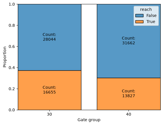

Does changing the first gate affect total rounds played?

We will be doing a Wilcoxon rank sum test (or Mann Whitney U) to see whether sum_gamerounds from gate_30 or gate_40 came from the same distribution. Basically, whether they are identical or not.

\(H_0\): Distribution of both samples are identical

\(H_1\): Distribution of both samples are NOT identical.

df_clean.groupby(by='version')[['version', 'sum_gamerounds']].describe()

	sum_gamerounds
	count	mean	std	min	25%	50%	75%	max
version
gate_30	44699.0	51.342111	102.057598	0.0	5.0	17.0	50.0	2961.0
gate_40	45489.0	51.298776	103.294416	0.0	5.0	16.0	52.0	2640.0

We can see that the mean is pushed because of the right tail, In fact, the mean is at 75th percentile of the data. I think it is wise to not rely on the mean to test whether these two versions are different.

# Wilcoxon rank sum test or Mann-whitney u test
round_30 = df_clean[df_clean['version'] == 'gate_30']['sum_gamerounds']
round_40 = df_clean[df_clean['version'] == 'gate_40']['sum_gamerounds']

u, p_val = stats.mannwhitneyu(round_30, round_40, alternative='two-sided')
print(f"u = {u:.3f}, p = {p_val:.4f}")

u = 1024285761.500, p = 0.0509

Although close, we failed to reject the null hypothesis where the two groups are the same as opposed to the alternative where there are difference in sum_gamerounds between the two groups with 95% significance. The test did almost reject however, leaning towards more total rounds played from gate 30 group.

We will be doing bootstrapping as well. We take 10000 samples from our data with replacement and take 3 different metrics to measure center.

Mean
Median
Trimmed mean

Because we know that we have a long tail on our distribution, we added median and trimmed mean as a way to check the robustness. Then, we will take the confidence interval for all three metrics. If the confidence interval includes 0, then the center of both distributions are indistinguishable.

# Bootstrapping
rng = np.random.default_rng(42)
sample_size = 10000
sample_mean, sample_median, sample_trimmed_mean = [], [], []

br30 = round_30.to_numpy()
br40 = round_40.to_numpy()

n30 = len(round_30)
n40 = len(round_40)

for i in range(sample_size):
    r30_sample = rng.choice(br30, size= n30, replace=True)
    r40_sample = rng.choice(br40, size= n40, replace=True)

    sample_mean.append(r30_sample.mean() - r40_sample.mean())
    sample_median.append(np.median(r30_sample) - np.median(r40_sample))
    sample_trimmed_mean.append(stats.trim_mean(r30_sample, 0.1) - stats.trim_mean(r40_sample, 0.1))

lo, hi = np.percentile(sample_mean, [2.5, 97.5])
print(f"Mean diff: {br30.mean() - br40.mean():+.3f}  95% CI [{lo:+.3f}, {hi:+.3f}]"
          f"  {'excludes' if lo > 0 or hi < 0 else 'includes'} 0")

lo, hi = np.percentile(sample_median, [2.5, 97.5])
print(f"Median diff: {np.median(br30) - np.median(br40):+.3f}  95% CI [{lo:+.3f}, {hi:+.3f}]"
          f"  {'excludes' if lo > 0 or hi < 0 else 'includes'} 0")

lo, hi = np.percentile(sample_trimmed_mean, [2.5, 97.5])
print(f"Trimmed mean diff: {stats.trim_mean(br30, 0.1) - stats.trim_mean(br40, 0.1):+.3f}  95% CI [{lo:+.3f}, {hi:+.3f}]"
          f"  {'excludes' if lo > 0 or hi < 0 else 'includes'} 0")

Mean diff: +0.043  95% CI [-1.288, +1.343]  includes 0
Median diff: +1.000  95% CI [+0.000, +1.000]  includes 0
Trimmed mean diff: +0.040  95% CI [-0.659, +0.733]  includes 0

The bootstrap agrees, all three metrics include 0. The median is a bit iffy due to discreteness of the metric, but the conclusion is still the same.

combined_df = pd.DataFrame({
    "value": sample_mean + sample_median + sample_trimmed_mean,
    "metric": ["sample_mean"]* sample_size + ["sample_median"] * sample_size + ["sample_trimmed_mean"] * sample_size
})

g = sns.FacetGrid(data= combined_df, row="metric", aspect=2, sharey=False, sharex=False)
g = g.map(sns.kdeplot, "value")
plt.show()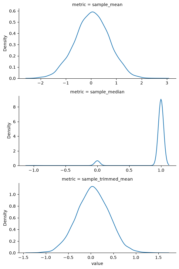

Both mean and trimmed mean are centered around zero, they just have different scale.

Does starting at different level affect retention?

We will be doing two proportion z-test to check. Basically checking whether the samples proportion for both gate 30 and gate 40 are the same for retention_1 and retention_7.

\(H_0\): Proportion of two samples are equal

\(H_1\): Proporiton of two samples are NOT equal

Retention 1

ret1_30 = df_clean[df_clean['version'] == 'gate_30']['retention_1']
ret1_40 = df_clean[df_clean['version'] == 'gate_40']['retention_1']

count1 = np.array([ret1_30.sum(), ret1_40.sum()])
nobs1  = np.array([ret1_30.count(), ret1_40.count()])

z_stat1, p_value1 = proportions_ztest(count1, nobs1, alternative='two-sided')
print(f"z = {z_stat1:.4f}, p = {p_value1:.4f}")

z = 1.7871, p = 0.0739

We fail to reject, meaning we do not have significant evidence that the two groups of gate_30 and gate_40 are not identical in terms of retention_1 according to this test.

Recall that we do not have a lot of players that actually reached the gate. Hence, we will be finding the Minimum Detectable Effect to confirm whether the two groups are identical, or we do not have enough sample size to detect differences. We will be taking MDE at the conventional 80% power and use retention rate as baseline.

h1 = NormalIndPower().solve_power(
    nobs1 = n30, alpha= 0.05, power= 0.8, ratio=n40/n30, alternative='two-sided'
)
phi1 = np.arcsin(np.sqrt(ret1_30.mean()))
p40_at_mde1 = np.sin(phi1 - h1 / 2) ** 2
mde1 = ret1_30.mean() - p40_at_mde1

print(f"baseline {ret1_30.mean():.4f} | observed {(ret1_30.mean() - ret1_40.mean())*100:+.2f} pp | "
          f"MDE {mde1*100:.2f} pp")

baseline 0.4482 | observed +0.59 pp | MDE 0.93 pp

The observed is lower than the MDE, meaning the experiment could only reliably detect changes for retention_1 of about .93pp. We would need more sample size.

Retention 7

ret7_30 = df_clean[df_clean['version'] == 'gate_30']['retention_7']
ret7_40 = df_clean[df_clean['version'] == 'gate_40']['retention_7']

count7 = np.array([ret7_30.sum(), ret7_40.sum()])
nobs7  = np.array([ret7_30.count(), ret7_40.count()])

z_stat7, p_value7 = proportions_ztest(count7, nobs7, alternative='two-sided')
print(f"z = {z_stat7:.4f}, p = {p_value7:.4f}")

z = 3.1574, p = 0.0016

We reject the null hypothesis and say that there is a significant evidence the two samples are different.

print(f"gate_30: {ret7_30.mean():.4f}   gate_40: {ret7_40.mean():.4f}   "
      f"diff: {ret7_30.mean() - ret7_40.mean():+.4f}")

gate_30: 0.1902   gate_40: 0.1820   diff: +0.0082

In fact, changing the gate to level 40 decreases the retention at 7th day.

h7 = NormalIndPower().solve_power(
    nobs1 = n30, alpha= 0.05, power= 0.8, ratio=n40/n30, alternative='two-sided'
)
phi7 = np.arcsin(np.sqrt(ret7_30.mean()))
p40_at_mde7 = np.sin(phi7 - h7 / 2) ** 2
mde7 = ret7_30.mean() - p40_at_mde7

print(f"baseline {ret7_30.mean():.4f} | observed {(ret7_30.mean() - ret7_40.mean())*100:+.2f} pp | "
          f"MDE {mde7*100:.2f} pp")

baseline 0.1902 | observed +0.82 pp | MDE 0.73 pp

The observed exceeds the MDE, meaning that the test could reliably detect effects.

# Binomial 95% CI
mean_diff1 = (ret1_30.mean() - ret1_40.mean())*100
ci1 = 1.96 * np.sqrt( ((sum(ret1_30)/len(ret1_30) * (1-sum(ret1_30)/len(ret1_30)))/len(ret1_30)) + 
            ((sum(ret1_40)/len(ret1_40) * (1-sum(ret1_40)/len(ret1_40)))/len(ret1_40))) * 100

mean_diff7 = (ret7_30.mean() - ret7_40.mean())*100
ci7 = 1.96 * np.sqrt( ((sum(ret7_30)/len(ret7_30) * (1-sum(ret7_30)/len(ret7_30)))/len(ret7_30)) + 
            ((sum(ret7_40)/len(ret7_40) * (1-sum(ret7_40)/len(ret7_40)))/len(ret7_40))) * 100

fig, ax = plt.subplots(figsize=(6, 2))
ax.errorbar(mean_diff7, 0, xerr=ci7, fmt='o', capsize=4)
ax.errorbar(mean_diff1, 1, xerr=ci1, fmt='o', capsize=4)

labels = ['7th Day (Primary)', '1st Day']
ax.set_yticks(range(len(labels)), labels)

ax.spines[['top', 'right']].set_visible(False)
ax.set_ylim(-0.5, 2 - 0.5)
ax.set_xlabel('Difference in retention, gate 30 − gate 40 (percentage points)')
ax.set_ylabel("Retention")
plt.tight_layout()
plt.show()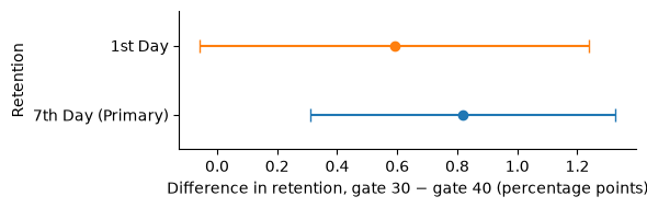

Visualization of the test

Conclusions and Recommendations

Due to the faultiness of the design of this test, alluding to the missed 50/50 sampling (from SRM test with chi2 = 6.902, p = 0.0086), we could not derive a strong recommendation. We could not investigate nor solve this issue because this is a public dataset. Therefore, be warned that the design may introduce bias and might affect results.

In terms of total rounds played, we did not detect a difference between gate 30 and gate 40 groups (from Wilcoxon Rank Sum test with p = 0.0509) the result leans toward more total rounds played from gate 30 group. The bootstrap results also agrees with mean difference of +0.043 and 95% CI of [-1.288, +1.343]. It is robust to trimming as well.

The retention on the 1st day for both group are not proven to be different (from two proportion z-test with z = 1.7871, p = 0.0739). This result however, is stated by the MDE as ‘undetectable change’ due to sample size not being enough (observed +0.59 pp | MDE 0.93 pp). One of the reasons is the samples being diluted by players that did not reach their intended gate for both groups by at least, two-thirds of the samples. On top of that, the total game rounds are calculated from the first 14 days, so that suggests even more dilution since there will be far fewer players that reached their intended gate within the first day.

Retention on the 7th day shows that moving the gate to level 40 decreases the retention (from two proportion z-test with z = 3.1574, p = 0.0016). It is a reliably detected effect but it is small.

Finally, our recommendations from this A/B test is as follows. We recommend to redo the experiment and redo the analysis to get a much stronger guidance. If we stick with this sample however, we could not recommend moving the gate to level 40, due to lowering the retention on the 7th day despite the shaky reliability. Not to mention, we did not detect any significant difference in other metrics as well.